Convolutional Neural Network from Scratch

2023-01-31

Contents

• Introduction
• A Simple Dataset
• Forward Propagation
• Backpropagation Overview
• Kernel Gradient
• Bias Gradient
• Input Gradient
• Implementing the Rest
• Flatten Layer
• Evaluation

Introduction

Previously, we had implemented a regular neural network, but this time we will step it up a notch by creating a convolutional neural network. But before we begin, I’m going to set a prerequisite for this blogpost. I want you to watch 3B1B’s video on convolutions first before you continue with this video on convolutions. Specifically, I want you to know at least what the computation of a cross-correlation and convolution looks like and also you should know what the difference is between those two operations. If you have at least a rough idea, you can continue. If not, you can still continue, but at some moments it might not click for you as much as it would have, if you watched 3B1B’s video first. Before we get into the nitty-gritty details of a convolutional layer, we first have to look at our dataset and in the previous episodes, I had used the MNIST dataset, but to make the derivations of the math simpler, I’m going to create a custom dataset.

A Simple Dataset

In general, our dataset will be a numpy tensor with this shape $x: [n \times c_{in} \times h \times w]$ where $n$ is the batch size, $c_{in}$ is the number of input channels (we’ll get to those later) and $H$ and $W$ are the height and the width of the input image. The input channel (at least in the case of image processing) often refers to the number of colour channels. For example, a grey-scaled image has only a single channel, which gives us the darkness of any pixel. A colour image would have 3 channels, one for the red, green and blue value of a pixel. In our simple dataset, we’re only going to have a single channel.

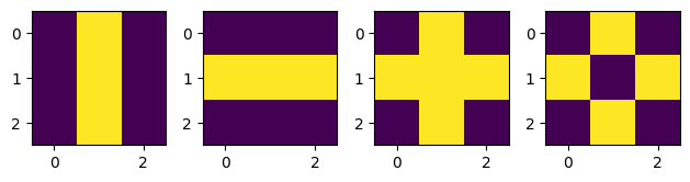
Our networks task will be to detect shapes. Here, I’ve predefined a couple of blueprints for the shapes and their corresponding target values.

V_LINE = np.array([[0, 1, 0], [0, 1, 0], [0, 1, 0]]).reshape(C_IN, H, W)
H_LINE = np.array([[0, 0, 0], [1, 1, 1], [0, 0, 0]]).reshape(C_IN, H, W)
CROSS = np.clip(V_LINE + H_LINE, a_min=0, a_max=1).reshape(C_IN, H, W)
DIAMOND = np.array([[0, 1, 0], [1, 0, 1], [0, 1, 0]]).reshape(C_IN, H, W)

_, (ax1, ax2, ax3, ax4) = plt.subplots(1, 4) # 1 row, 4 columns


ax1.imshow(np.array([[0, 1, 0], [0, 1, 0], [0, 1, 0]]))
ax2.imshow(np.array([[0, 0, 0], [1, 1, 1], [0, 0, 0]]))
ax3.imshow(np.clip(np.array([[0, 1, 0], [0, 1, 0], [0, 1, 0]]) + np.array([[0, 0, 0], [1, 1, 1], [0, 0, 0]]), a_min=0, a_max=1))
ax4.imshow(np.array([[0, 1, 0], [1, 0, 1], [0, 1, 0]]))

plt.tight_layout()


SHAPES = {
    "v_line":V_LINE,
    "h_line": H_LINE,
    "cross": CROSS,
    "diamond": DIAMOND
}
TARGETS = {
    "v_line":0,
    "h_line": 1,
    "cross": 2,
    "diamond": 3
}

Our dataset will consist of these, but not exactly these, because our network would easily just memorise these values. Instead, we will use these as a blueprint and add a bit of random noise on top to make sure that our network doesn’t just simply memorise these numbers.

def generate_single_data_point(shape: str):
    return TARGETS[shape], (SHAPES[shape] + np.random.uniform(-0.25, 0.25, size=(C_IN, H, W)))

def generate_dataset(n=500, batch_size=16):
    def split_into_batches(x, batch_size):
        n_batches = len(x) / batch_size
        x = np.array_split(x, n_batches)
        return np.array(x, dtype=object)
    one_hot_encoder = OneHotEncoder()

    shapes = list(SHAPES.keys())
    dataset = [generate_single_data_point(np.random.choice(shapes)) for _ in range(n)]
    labels = []
    data = []
    for y, x in dataset:
        labels.append(y)
        data.append(x)

    targets = np.array(labels)
    data = np.array(data)
    X_train, X_test, y_train, y_test = train_test_split(data, targets, test_size=0.33, random_state=RANDOM_SEED)

    X_train = split_into_batches(
        X_train, batch_size
    )

    X_test = split_into_batches(
        X_test, batch_size
    )

    # Turn the targets into Numpy arrays and flatten the array
    y_train = np.array(y_train).reshape(-1, 1)
    y_test = np.array(y_test).reshape(-1, 1)

    # One-Hot encode the training data and split it into batches (same as with the training data)
    one_hot_encoder.fit(y_train)
    y_train = one_hot_encoder.transform(y_train).toarray()
    y_train = split_into_batches(np.array(y_train), batch_size)

    one_hot_encoder.fit(y_test)
    y_test = one_hot_encoder.transform(y_test).toarray()
    y_test = split_into_batches(np.array(y_test), batch_size)

    return X_train, y_train, X_test, y_test

This function generate_dataset(...) basically generates 500 datapoints with their corresponding, one-hot encoded target values and then splits the data into a training and testing set. I won’t go into detail what this function does, because the exact procedure of this function doesn’t really matter to us right now. Also you don’t need any machine learning knowledge to understand this code, so if you want to, you can look at this later on your own free time. For now, we’ll treat this as a blackbox that simply generates the dataset for us.

Now that we have the data, we can finally start with forward propagation.

Forward Propagation

As mentioned before, on this left side, we have our input data with the familiar shape. Note that each of these boxes is a whole matrix. In the middle, we have the heart of our convolutional layer, namely the kernels and the biases, which represent the trainable parameters of the convolutional layer. We call each column here a kernel, and each kernel consists of a set of matrices and a single bias value. Each kernel has as many matrices as we have input channels and we will see why that is the case in just a moment. The number of kernels defines the shape of the output of the convolutional layer and that number is called $c*{out}$ or the number of output channels. And since each kernel matrix is a squared matrix (which is doesn’t have to be, I just like it this way), the final shape of the kernels is $[c*{out} \times c_{in} \times t \times t]$ . We also have the bias matrix, which is just a single row matrix. We use this comma notation, to tell numpy to perform broadcasting and I’ve covered broadcasting in my previous blogposts.

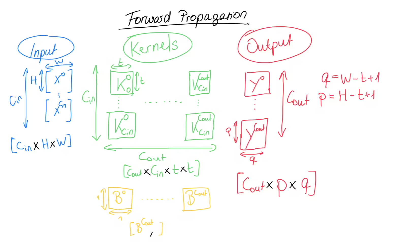
The output of the convolutional layer is another set of matrices. While the input had $c*{in}$ as the number of channels, for our output, the number of channels is $c*{out}$ . Also, each box here is a matrix, with the shape $p \times q$ />, and these values depend on the width and height of our input matrices as well as our kernels. More specifically, what you see here is the resulting shape of a so-called valid cross-correlation between two matrices.

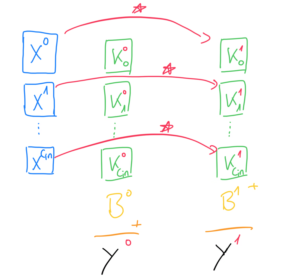
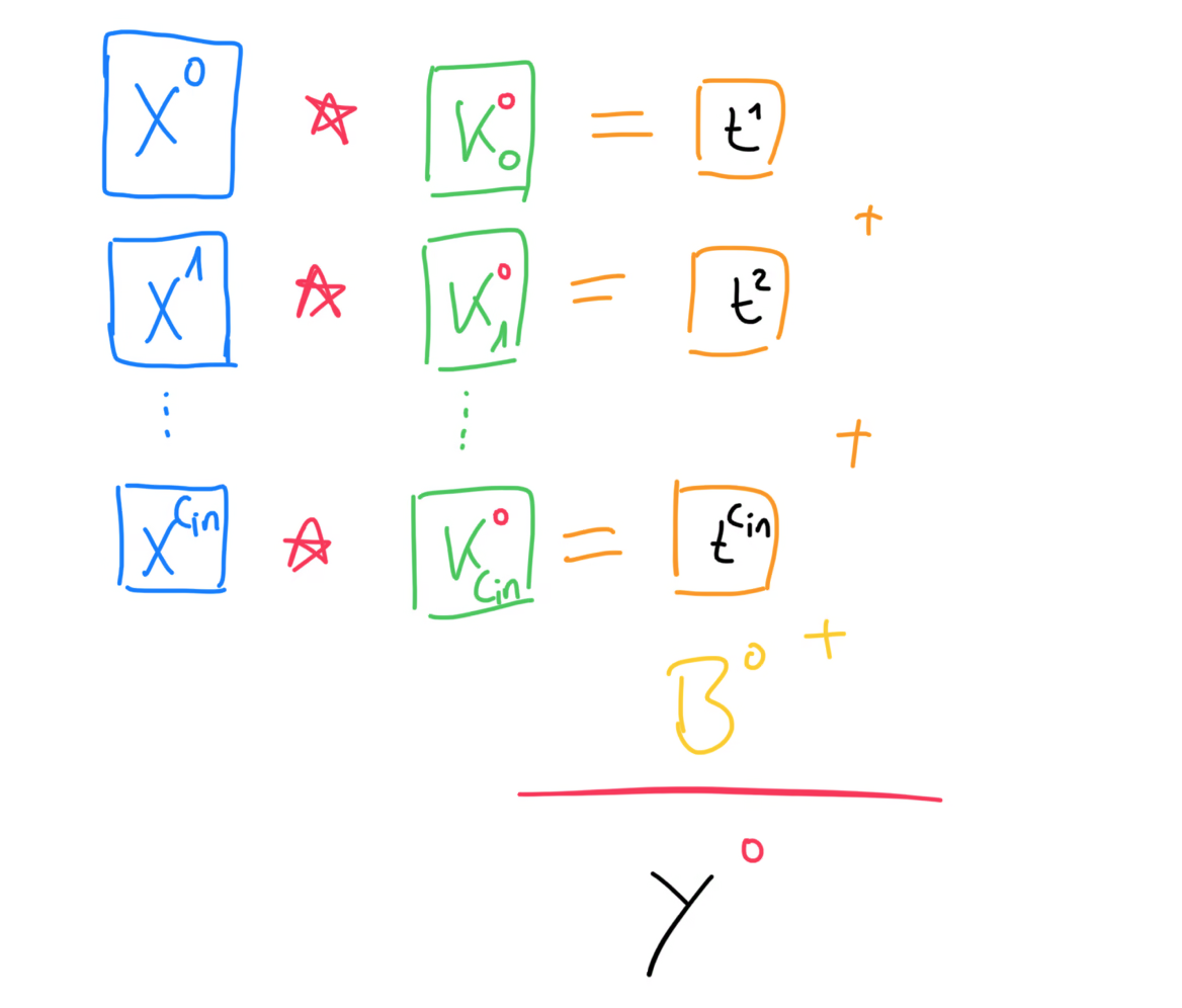
For the actual forward propagation, we will take each of the input channel matrices and compute the cross-correlation between them and the matrices of the first kernel. Now you should see why each kernel must have exactly $c_{in}$ matrices, because each channel of the input needs to be cross-correlated with a kernel matrix. Then, we take the sum of each of these cross-correlations and add the bias on top. Remember, that the bias is a single number, but that’s fine, since numpy will perform broadcasting for us and that single number will be added to every value of the matrix. The result of all of this is the first of the output matrices. We then repeat this process for every kernel.

More generally, we can write the formula for the forward propagation like this. This is where we have to bring back our batch size, that we omitted in the beginning. This forward propagation step has to be performed for every training example in the batch, which means we have to iterate over our batch and then perform forward propagation for every datapoint.

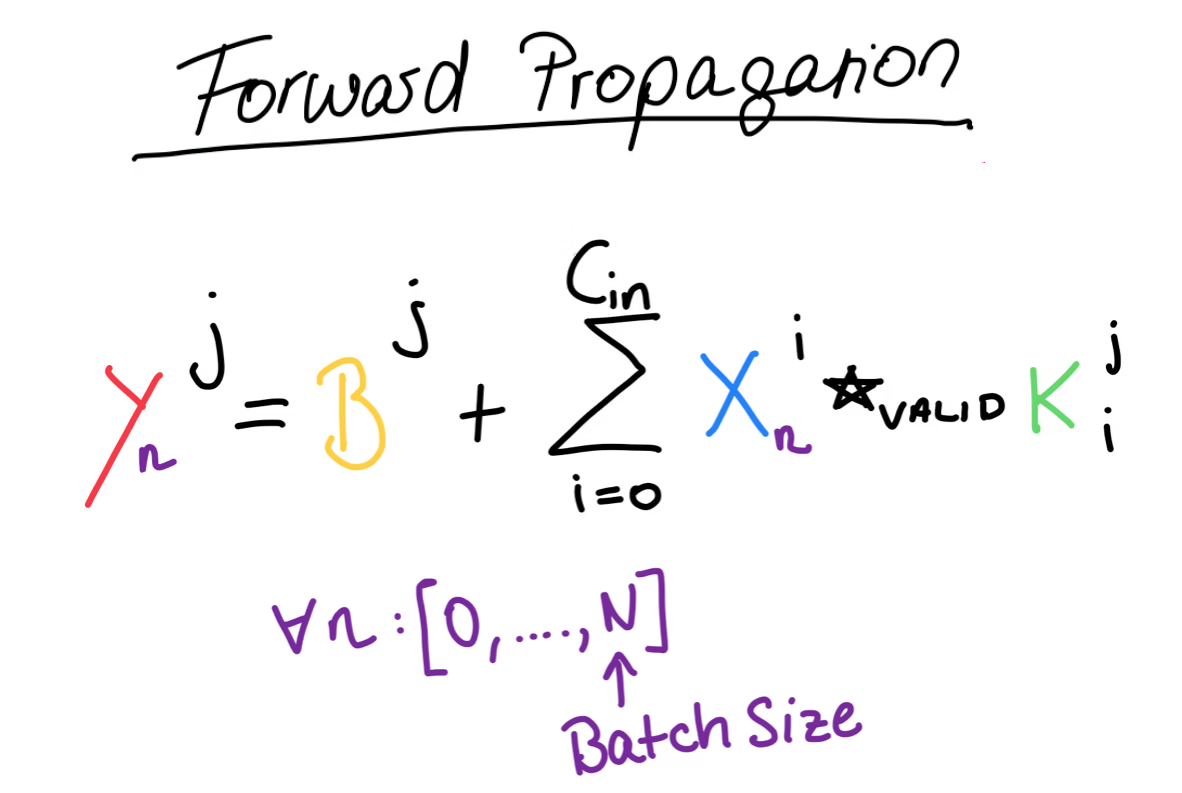
Let’s implement this in Python.

def conv2d_forward(x: np.array, kernels: np.array, bias: np.array):
    c_out, c_in, k, _ = kernels.shape
    N, c_in, h_in, w_in = x.shape
    h_out = h_in - k + 1
    w_out = w_in - k + 1
    output_shape = N, c_out, h_out, w_out
    output = np.zeros(shape=output_shape)
    for n in range(N):
        for j in range(c_out):
            output[n, j] = bias[j]
            for i in range(c_in):
                output[n, j] += correlate2d(
                    x[n, i], kernels[j, i], mode="valid"
                )
    return output

First we gather all the hyper parameters from our input. We can get the number of channels from the kernels and the batch size and the dimensions of the image from the input matrix. With that we initialise the empty output array. We then iterate over every sample in our batch and perform forward propagation pretty much exactly as we’ve written it in our formula. This correlate2d() function comes from SciPy and is a neat helper for us. In Numpy, there is only the “normal” cross-correlation which - in mathematical terms - is an operation between two functions, not necessarily between matrices. This function from ScipPy does this operation on 2d matrices, so we won’t have to implement that from scratch. Finally, we return the output.

This was it for the forward propagation step, but the difficult part is yet to come, which is the back propagation step in which we update the trainable parameters of our layers.

Backpropagation Overview

As always, we get as input the error gradient, which can either come from this layer being the output layer of the whole network, or our layer being just some layer in the middle, meaning we get it from the layer in front.

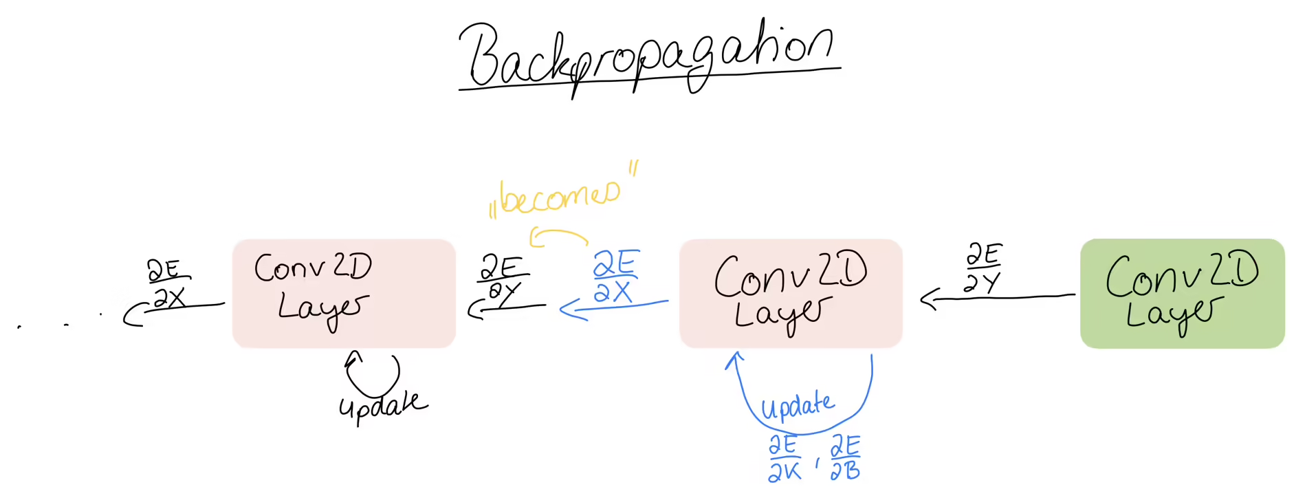
Either way, we have to use this error gradient to compute the partial derivatives for the kernel and the bias. Then, the output of the back propagation is the input error, which we pass to the layers before us. That input error then becomes the error gradient for the layer behind us. Then that layer computes the gradients and passes the error backwards and so on. So to summarise, we get the error gradient matrix as input and we have to compute the gradient matrices: the kernel gradient, the bias gradient and the input gradient. Let’s start with the kernel gradient.

Kernel Gradient

So far this is all the information we have:

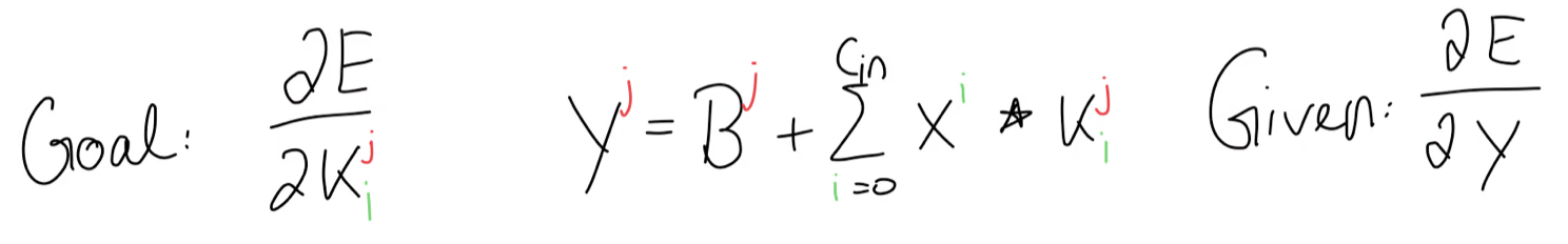
If we write out the forward propagation equation, we get this for $j=0$, or in other words, the first set of kernels.

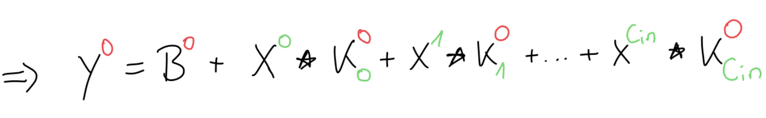
Our goal is to find a generic formula such that we can compute any arbitrary kernel gradient, for example this kernel gradient for $j=0$ and $i=1$. Since $j=0$, we look at the equation of $y$ where $j=0$. And although all of these terms here are matrices and we can’t use the chain rule directly, we can still use the general idea of the chain rule by asking ourselves, how much influence did $K_0^1$ have on the error gradient.

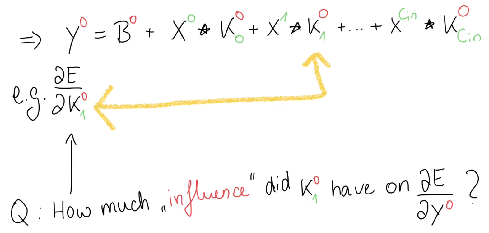
Well, we can see in this equation, that $K_0^1$ only appears once here. And, since we have a sum here, when we would take the derivative of this output, everything else would become $0$ anyway, except the part where our kernel had some influence. This means that the only relevant part of this equation, as far as $K_0^1$ is concerned, can be boiled down to this part:

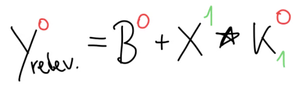
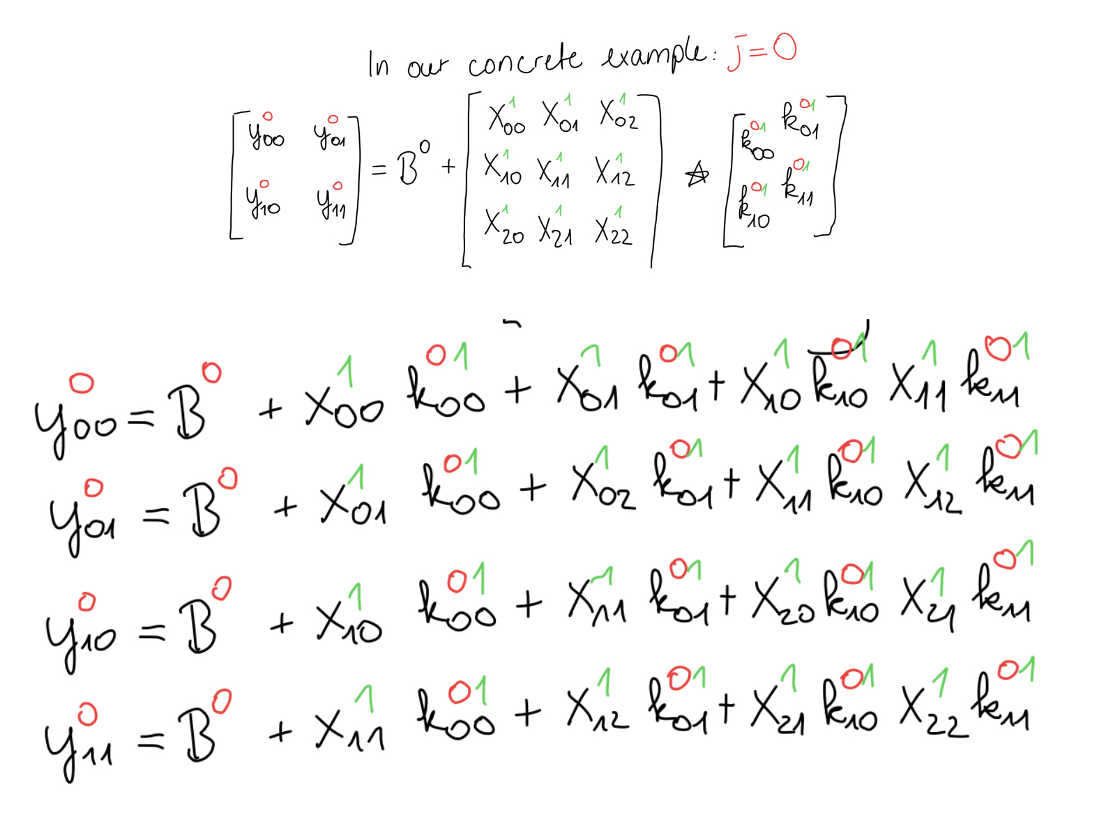
In our concrete example, with our parameters, this can be written like so in matrix form.

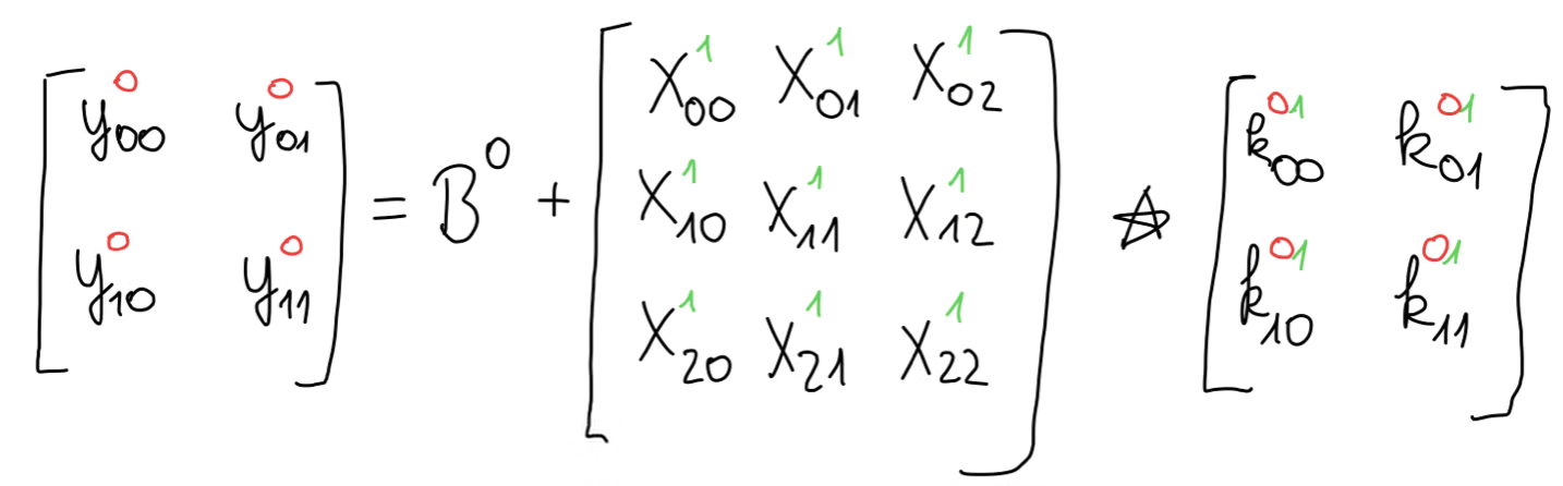
We can expand the equations of the cross-correlation, giving us this set of equations.

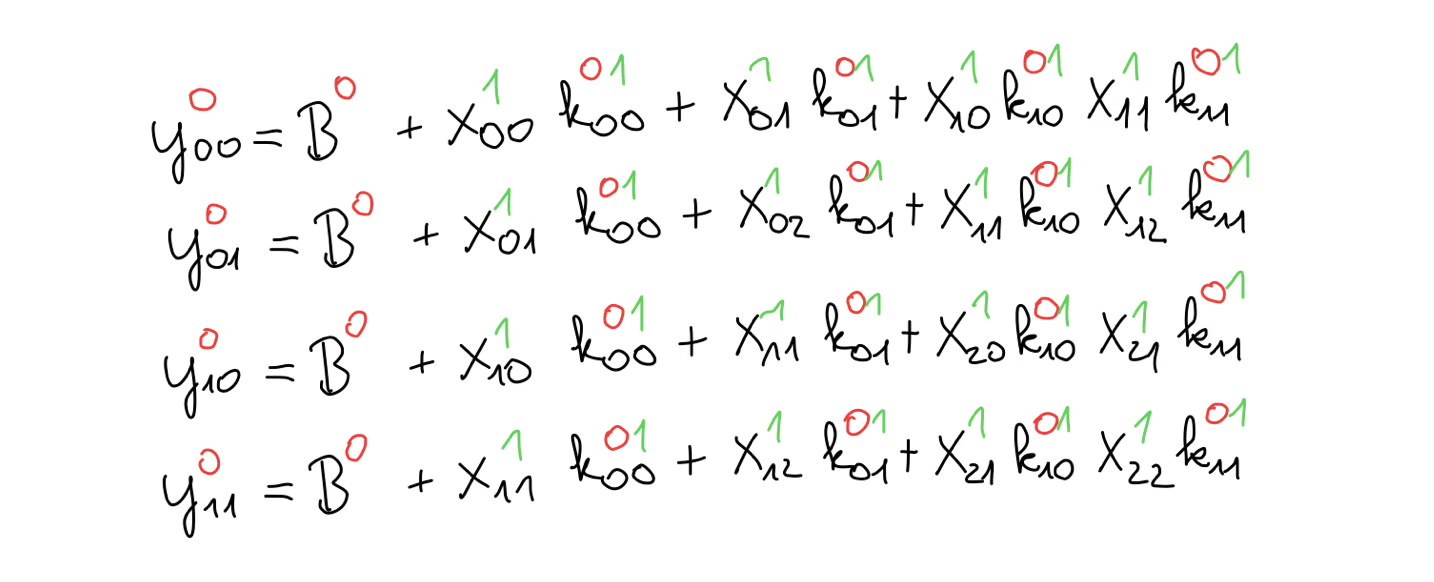
And, just to remind ourselves, our goal is to compute the kernel gradient given the output gradient.

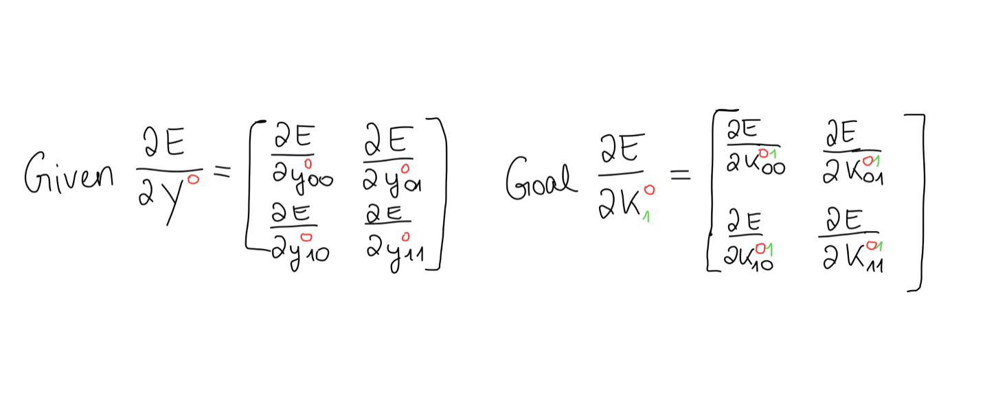
For this, we can use the chain rule. I know, this looks confusing, but once you break it down, it really isn’t.

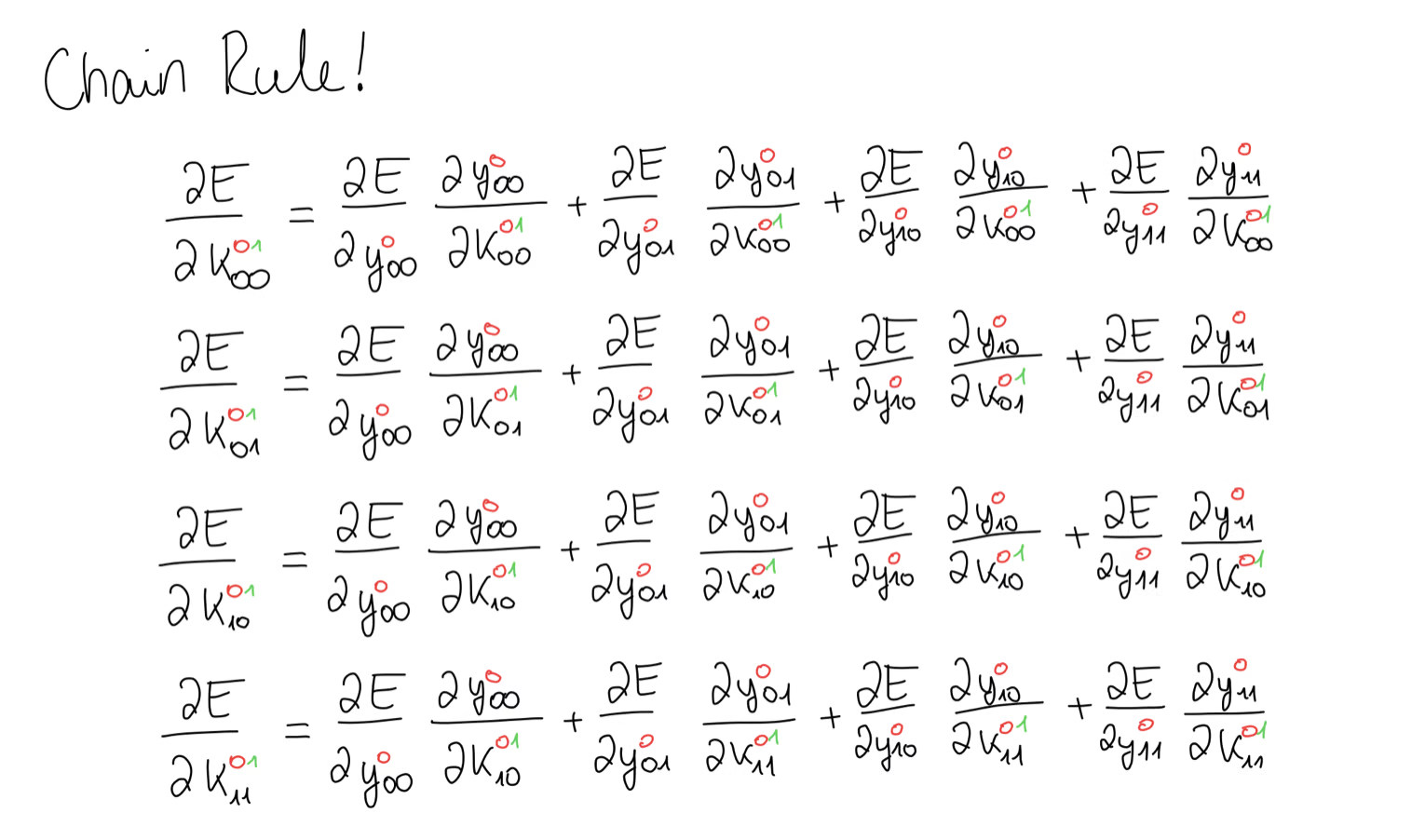
For example, in this first equation, we are looking for all the contributions of $K*{00}^{01}$ towards the error gradient. We notice, that $K*{00}^{01}$ appears in all 4 equations, meaning we have 4 contributions of $K_{00}^{01}$ and we have to add those up. The same goes for all the other values of the kernel. Lucky for us, these gradients are very easy to calculate and all we’re left with is some part of our input matrix $X$ .

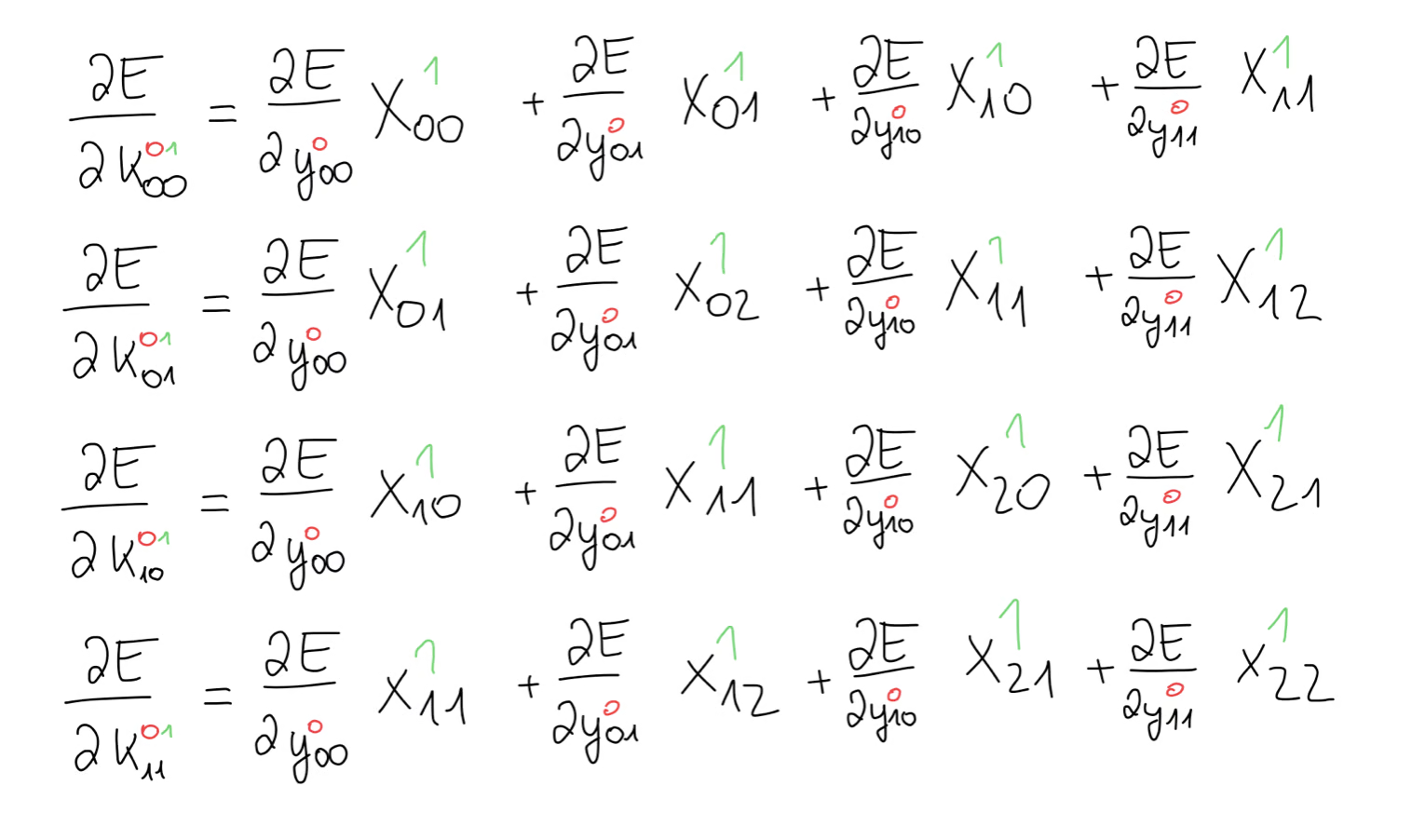
It looks as though we have some sort of operation between our input matrix and the error gradient.

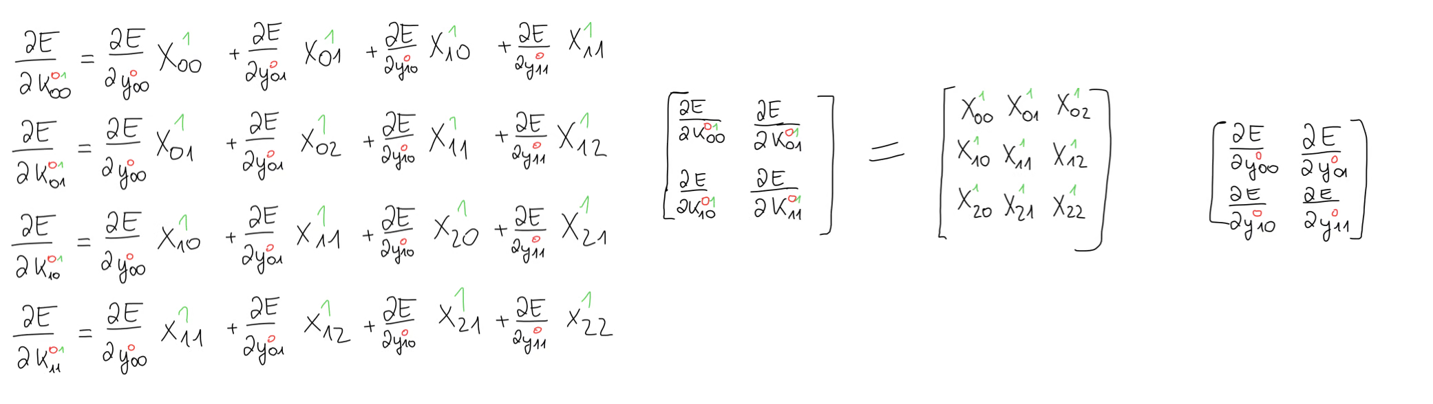
What we have here is the valid cross-correlation that we had previously used in the forward propagation step. At this point, it might help to take a moment to verify that this really is the cross-correlation operation.Now, we can bring this back to matrix form and taking this one step further, we can write the generic formula to compute any kernel gradient we want.

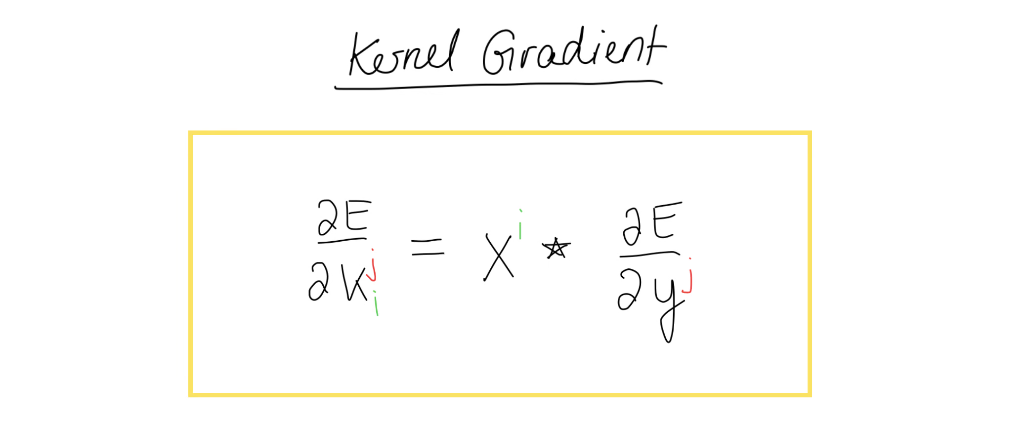
We can now take this formula and implement this in Python.

def conv2d_kernel_gradient(dE_dY: np.array, x: np.array):
    n, c_out, h_out, w_out = dE_dY.shape
    _, c_in, h_in, w_in = x.shape
    k = h_in + 1 - h_out
    dK = np.zeros(shape=(c_out, c_in, k, k))
    for batch in range(n):
        for i in range(c_out):
            for j in range(c_in):
                dK[i, j] += correlate2d(dE_dY[batch, i], x[batch, j], mode="valid")

    return dK / n

We once again first take all the necessary parameters from our inputs and we also reverse engineer what the shape of the kernels is. Then, we iterate over all our batches and compute the gradients exactly as in the formula. One extra step we have to take care of is that we’re adding up all the gradients from every training sample. In the end, we divide the kernel gradient by the batch size, which gives us the average kernel gradient. If we didn’t do this part, we would have one giant kernel gradient, but instead we want to have the average kernel gradient, which is why we divide this by the batch size in the end.

his was the kernel gradient. Next up is the bias gradient.

Bias Gradient

For the bias gradient we take the same approach as before. We write out the equation for the output and ask ourselves: how much influence did the bias have on the error gradient.

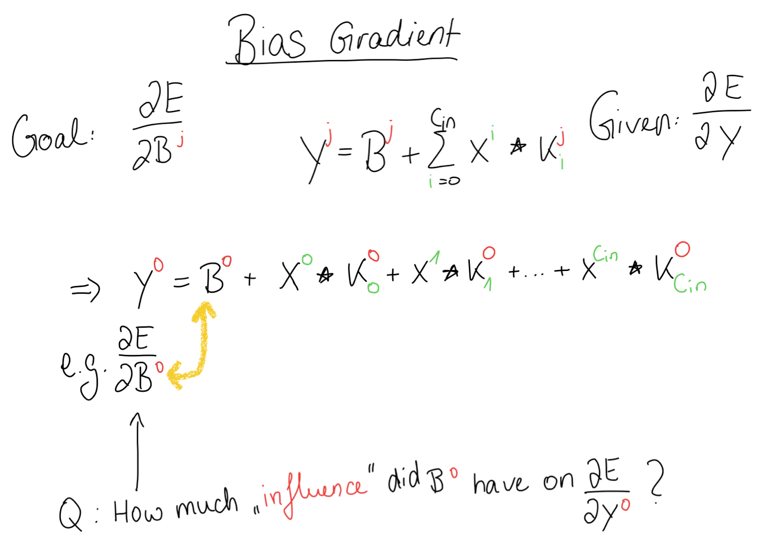
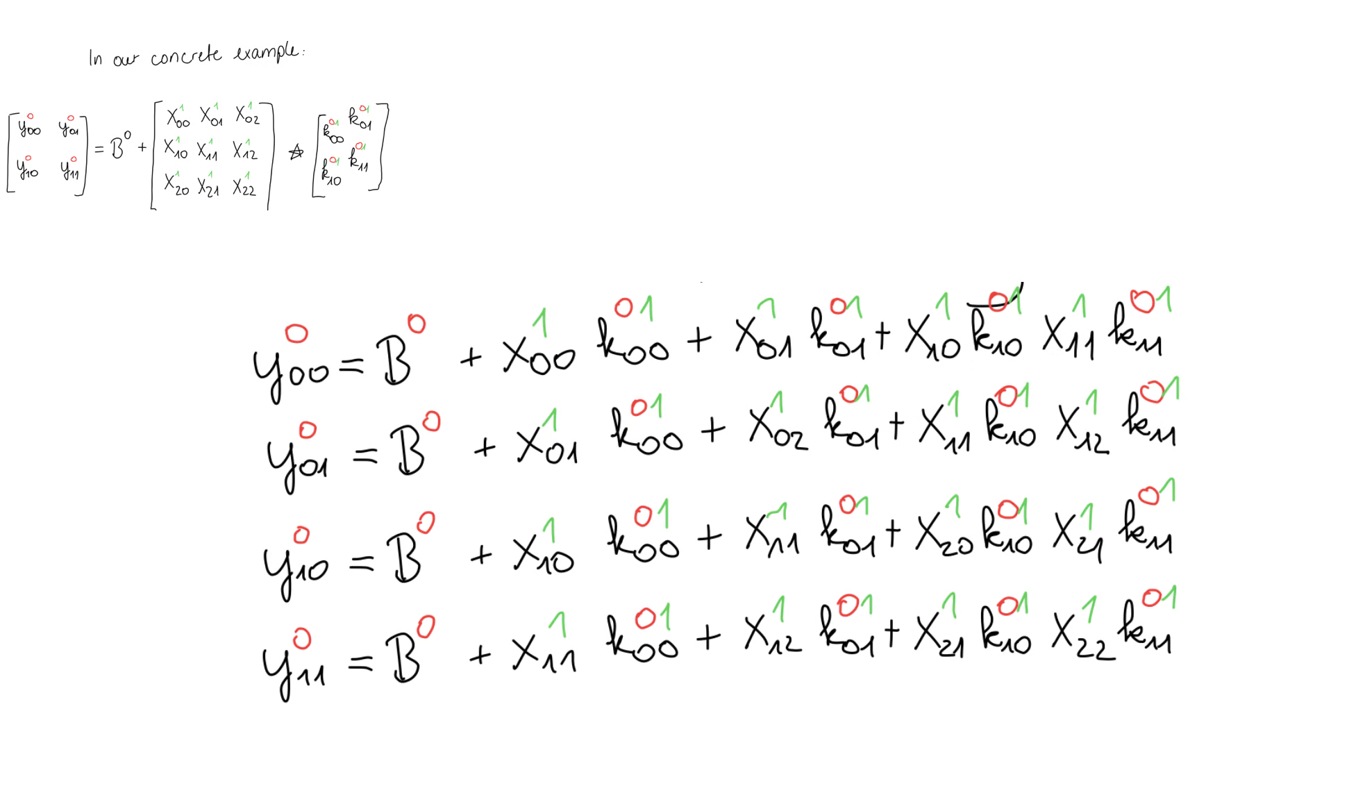
Then, we write out the forward propagation equation for our concrete example and also the equations that come from the cross-correlation operation, exactly as we did before. Again, our goal is to compute the bias gradient given the error gradient.

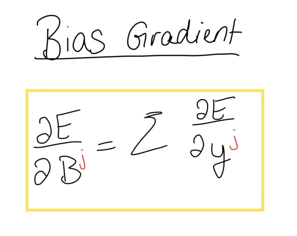
We notice that the bias appears in every equation, so we use the chain rule to write out the bias gradient. This time, all we’re left with is the error gradient, which means we have to take the sum of the error gradient.

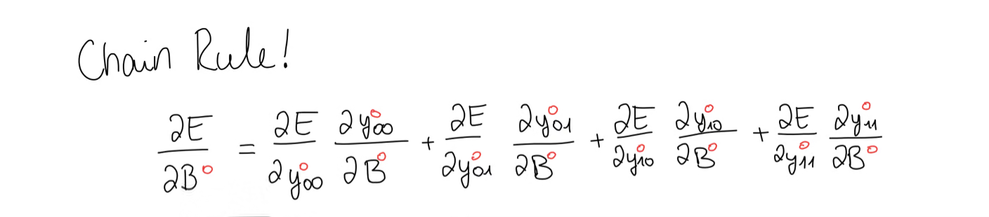
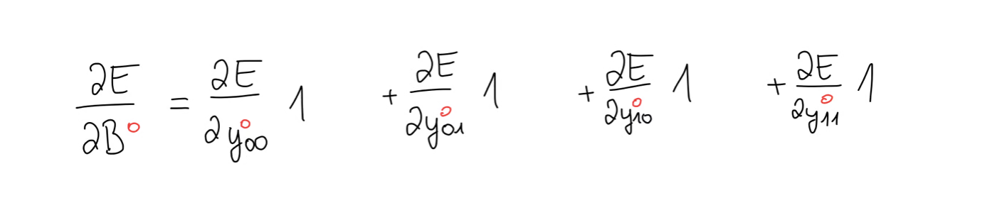
Depending on your case, it could be that the bias becomes really big in which case you might want to take the average. To summarise, the bias gradient is equal to the sum of the elements of the error gradient.

We can now implement this in Python.

def conv2d_bias_gradient(dE_dY: np.ndarray):
    n, c_out, _, _ = dE_dY.shape
    dB = dE_dY.sum(axis=(0, 2, 3)) / n
    return dB

This part is actually quite short, since all we have to do is use the sum function from numpy and give the first, third and fourth axis as input, meaning we take the sum of all axes, except for the one of the output channels. We do this, because the bias is a matrix with the shape of $c_{out}$. And using the sum function this way, we aggregate the values over this axis, giving us a matrix with the same shape as the axis that we left out, that is the same shape as the bias matrix.

Now that’s 2 out of 3 gradients done. The last one is a little more tricky, although not by much.

Input Gradient

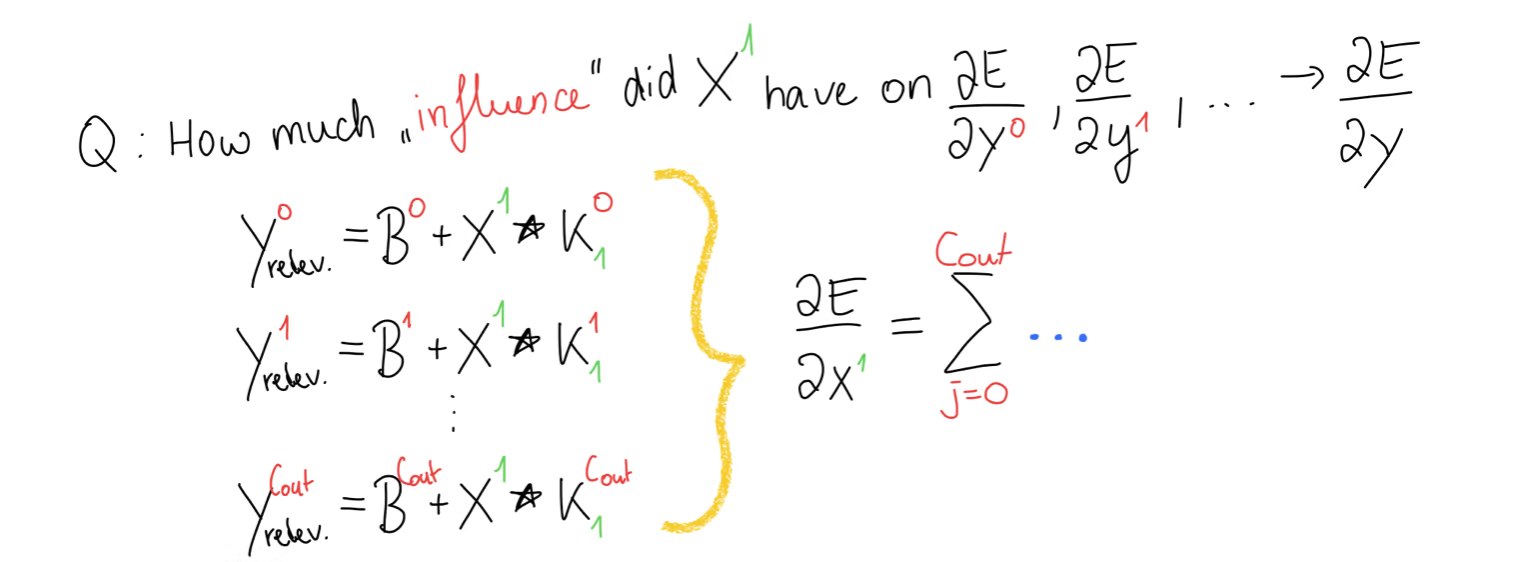
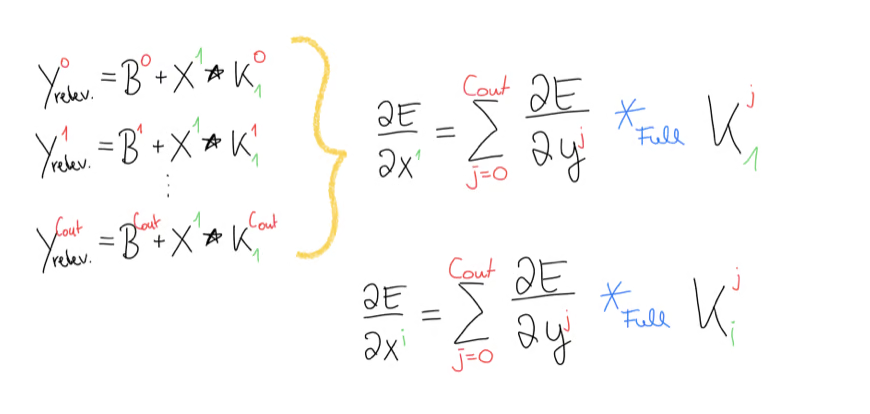
Our goal is to compute the input gradient and for that we have to figure out, where this input, for example $X^1$ appeared in our forward propagation. For that, we write out the equation. But we should know, that $X^1$ didn’t just appear in this output matrix but rather it appeared in every equation.

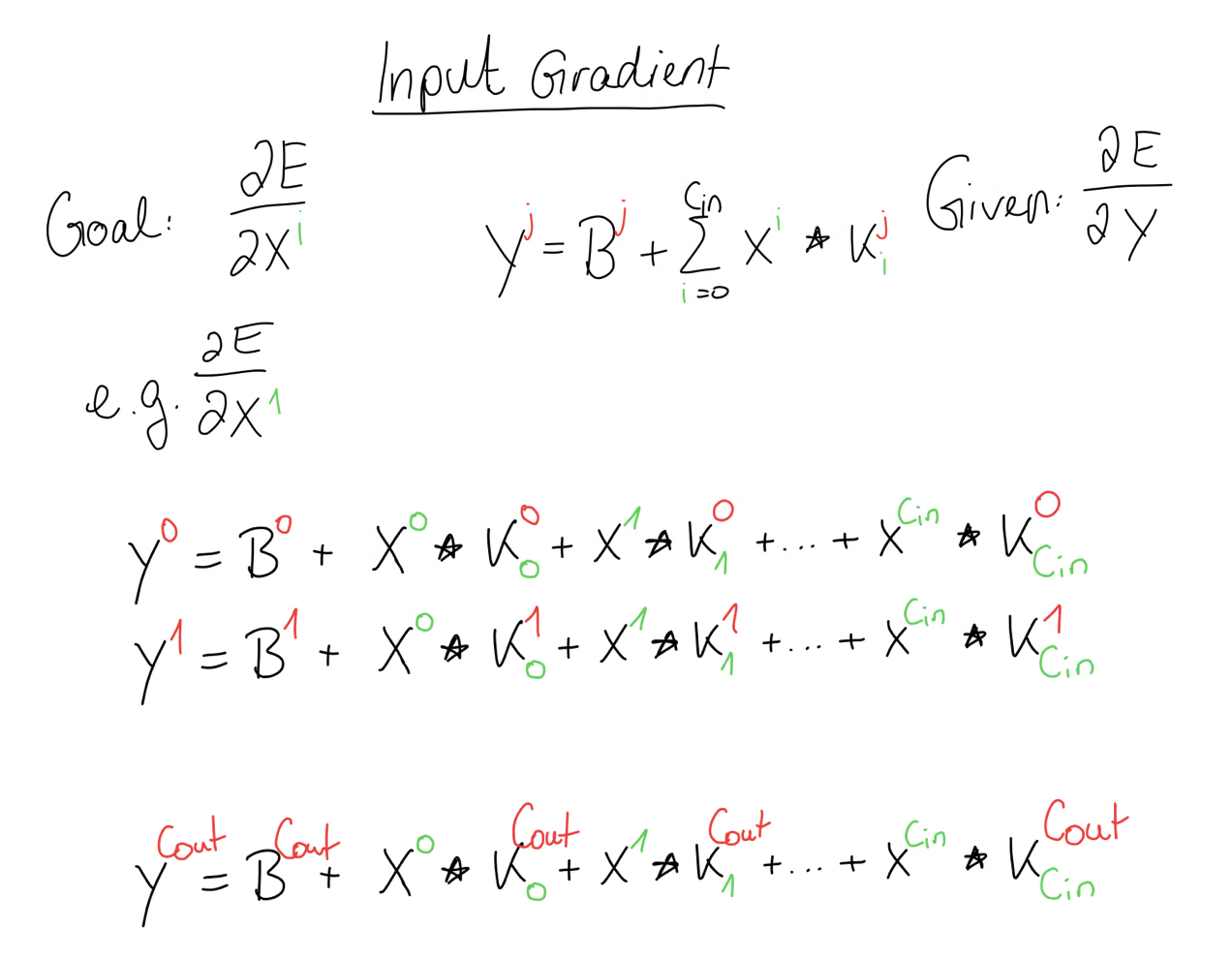
So while the relevant part still gets smaller, as every other value becomes $0$ when we take the gradient, we are still left with a set of equations. Meaning that in the end, to compute the gradient of $X^1$ , we will have some sort of loop that sums the contributions of $X^1$ from all the equations.

For now, let’s just focus on a single equation where $j=0$. We can write out the equations of the cross-correlation step like this.

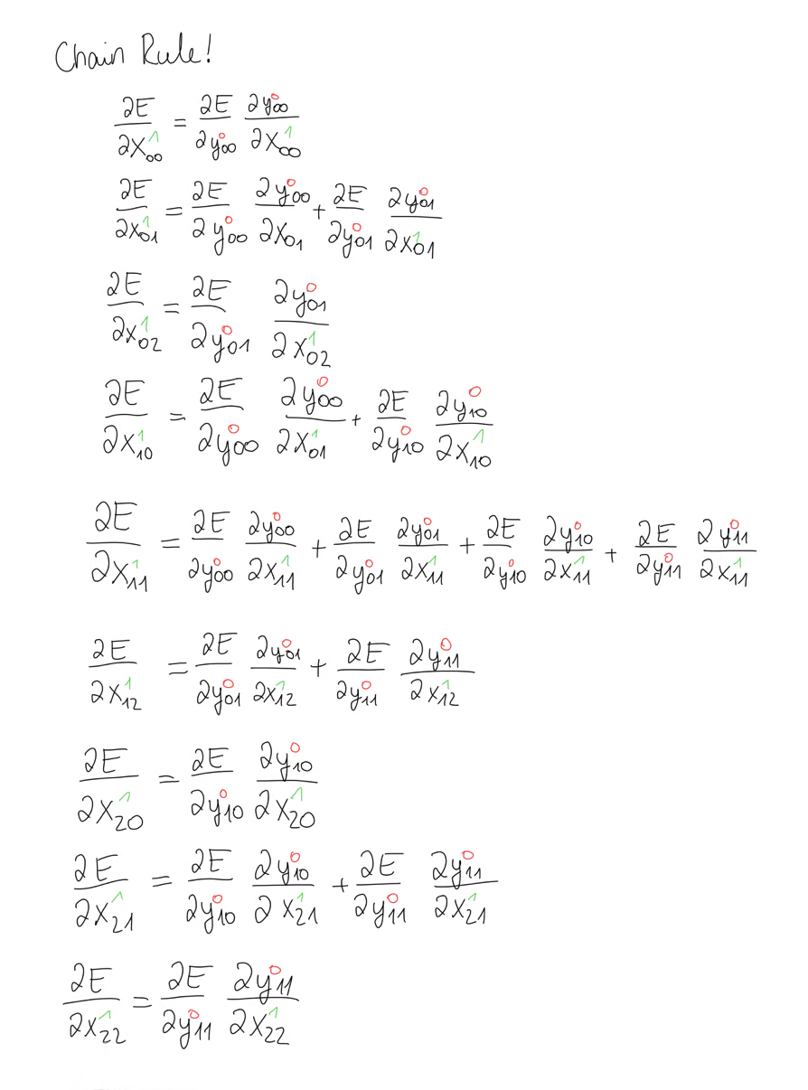
Again, our goal is to compute this input gradient matrix. For that we have to use the chain rule. Since our input matrix has 9 elements, we have 9 equations. We follow the same procedure as with the kernel gradient. For example, $X*{00}$ appears once in the first equation, meaning we have only a single contribution of $X*{00}$ the error. Another example is $X*{11}$. We see that $X*{11}$ appears in all 4 equations, meaning we have 4 contributions of <Katex math={“X_{11}”} and we have to add all those up. We follow this procedure for every element of $X$.

When we then compute the derivatives, we are left with the kernels. This means that we have some kind of operation between the error gradient and our kernel matrix.

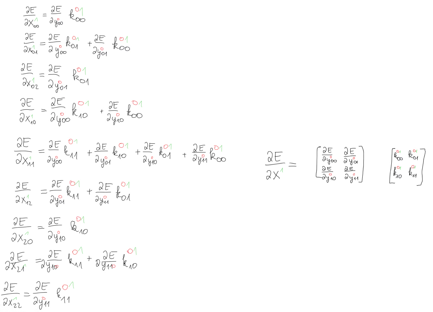
What this operation is is not so obvious on the first glance, but when we look at this equation for $X_{11}$, we notice that we have our kernel except that it’s rotated by 180 degrees.

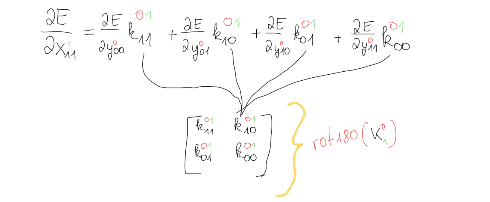
This gives us a hint that we might dealing with a convolution here but not just any convolution, but rather the full convolution, because the number of equations isn’t the same in every equation, which is should have been, if we had a valid convolution. And this is in fact correct, that the operation we’re looking for is the full convolution between the error gradient and the kernel.

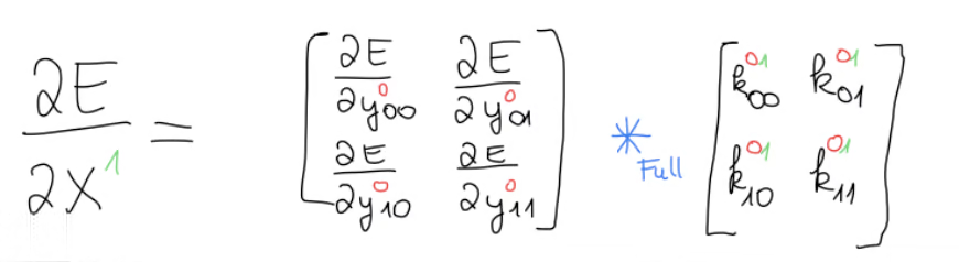
Now this is good and all, but we have to remember that $X^1$ appeared in every equation in the beginning and we had already noticed that in the end we will need some kind of sum over every $j$ in the range of $c_{out}$, giving us this equation. As the last step, we write the generic function such that we can compute any input gradient.

We can now implement this in Python.

def conv2d_input_gradient(dE_dY: np.ndarray, kernels: np.ndarray):
    n, c_out, h_out, w_out = dE_dY.shape
    c_out, c_in, k, _ = kernels.shape
    h_in = h_out + k - 1
    w_in = w_out + k - 1
    dX = np.zeros((n, c_in, h_in, w_in))

    for batch in range(n):
        for j in range(c_in):
            for i in range(c_out):
                dX[batch, j] += convolve2d(dE_dY[batch, i], kernels[i, j], mode="full")
    return dX

We again derive all the necessary parameters from our function inputs. Then, we have to iterate over every training sample in our batch and then write out the equation pretty much exactly as we had defined before.

Implementing the Rest

With that we are pretty much done with the convolutional layer. All that’s left is to implement the remaining network in Python. First we create two helpers to initialise our parameters.

def init_random_kernels(c_in, c_out, kernel_size):
    return np.random.randn(c_out, c_in, kernel_size, kernel_size)


def init_random_bias(c_out):
    return np.random.randn(c_out)

Then, we create a class called Conv2D, which holds the logic of our convolutional layer. We then implement the forward and backwards methods by using the functions we had defined before. Finally, in the update method, we take the gradients as input and perform the actual gradient descent step.

class Conv2D:
    def __init__(self, c_in, c_out, kernel_size) -> None:
        self.k = init_random_kernels(c_in, c_out, kernel_size)
        self.b = init_random_bias(c_out)

    def forward(self, x: np.ndarray):
        self.x = x
        return conv2d_forward(x, self.k, self.b)

    def backward(self, dE_dY: np.ndarray):
        dK = conv2d_kernel_gradient(dE_dY, self.x)
        dB = conv2d_bias_gradient(dE_dY)
        dX = conv2d_input_gradient(dE_dY, self.k)

        return {"dK": dK, "dB": dB, "dX": dX}

    def update(self, grads, learning_rate):
        self.k -= grads["dK"] * learning_rate
        self.b -= grads["dB"] * learning_rate

Flatten Layer

Before we can use the convolutional layer in a network, we need another layer, namely the flatten layer. This layer has no trainable parameters and all it does is to flatten the 2d convolutional layer into a single dimension.

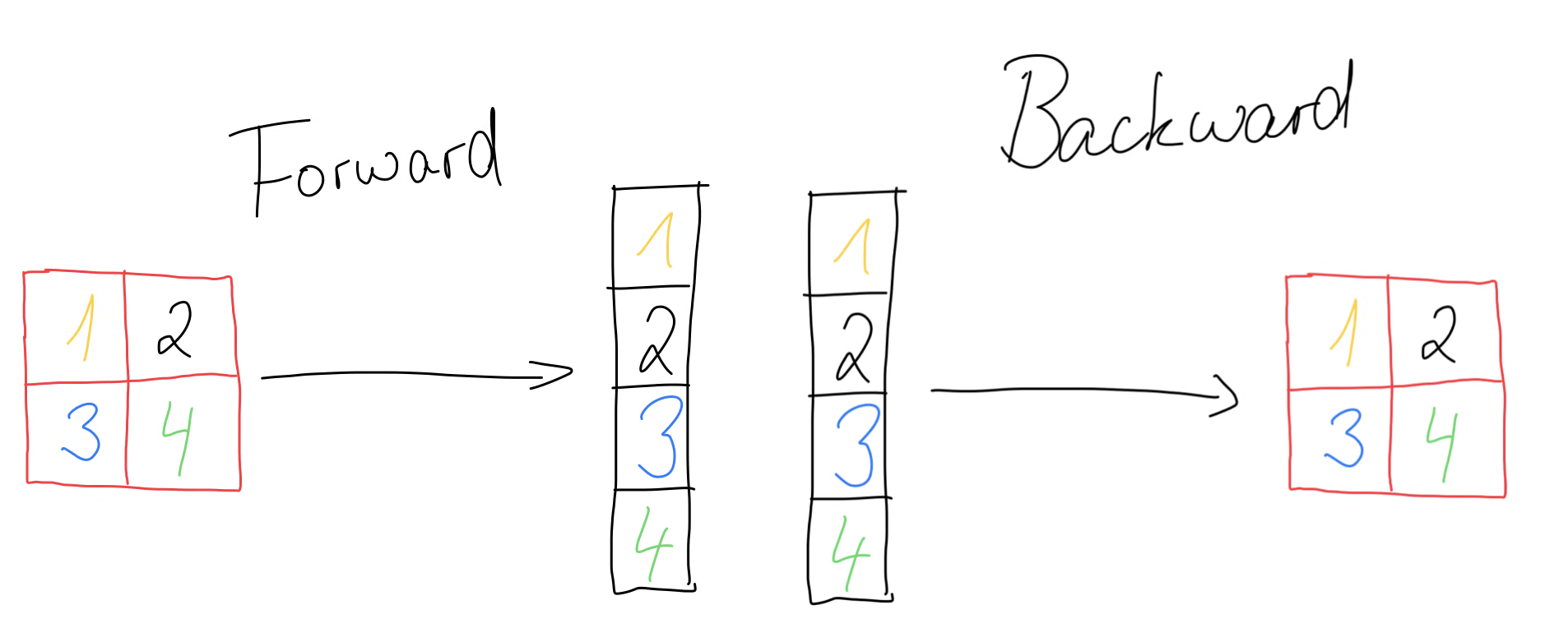
We can achieve this functionality by using the reshape method and passing it $-1$ as the second parameter. The backward method takes as input the error gradient and reshapes it back to its original form that it had during forward propagation. The update method won’t do anything, since we have no trainable parameters.

class Flatten:
    def __init__(self):
        self.x = None

    def forward(self, x: np.ndarray):
        self.x = x
        n = x.shape[0]
        return self.x.reshape((n, -1))

    def backward(self, dE_dY: np.ndarray):
        return {"dX": dE_dY.reshape(self.x.shape)}

    def update(self, grads, learning_rate):
        pass

We then need a couple of activation functions and a dense layer, both of which we take more or less directly from the previous blog posts, I won’t go into detail here.

def init_dense_layer(n_in, n_out) -> tuple[np.ndarray, np.ndarray]:
    w = np.random.randn(n_in, n_out) * 0.1
    b = (
        np.random.randn(
            n_out,
        )
        * 0.1
    )

    return w, b


def forward_single_dense_layer(x: np.ndarray, w: np.ndarray, b: np.ndarray):
    return x @ w + b


def get_weight_gradient_single_dense_layer(x: np.ndarray, dE_dY: np.ndarray):
    return x.T @ dE_dY


def get_bias_gradient_single_dense_layer(dE_dY: np.ndarray):
    return np.sum(dE_dY, axis=0) / dE_dY.shape[0]


def get_input_gradient_single_dense_layer(dE_dY: np.ndarray, w: np.ndarray):
    return dE_dY @ w.T

class ReLU:
    def __init__(self) -> None:
        self.x = None

    @staticmethod
    def relu(Z):
        return np.maximum(0, Z)

    @staticmethod
    def relu_backward(x):
        x[x <= 0] = 0
        x[x > 0] = 1
        return x

    def forward(self, x):
        self.x = x
        return self.relu(x)

    def backward(self, dE_dY):
        dX = np.multiply(dE_dY, self.relu_backward(self.x))
        return {"dX": dX}

    def update(self, *args, **kwargs):
        pass


class Sigmoid:
    def __init__(self):
        self.x = None
        pass

    @staticmethod
    def sigmoid(Z):
        return 1 / (1 + np.exp(-Z))

    @staticmethod
    def sigmoid_backward(x):
        sig = Sigmoid.sigmoid(x)
        return sig * (1 - sig)

    def forward(self, x):
        self.x = x
        return self.sigmoid(x)

    def backward(self, dE_dY):
        dX = np.multiply(dE_dY, self.sigmoid_backward(self.x))
        return {"dX": dX}

    def update(self, *args, **kwargs):
        pass


class Dense:
    def __init__(self, n_in, n_out) -> None:
        self.w, self.b = init_dense_layer(n_in, n_out)
        self.x = None

    def forward(self, x: np.ndarray):
        # print(x.shape)
        self.x = x
        return forward_single_dense_layer(self.x, self.w, self.b)

    def backward(self, dE_dY: np.ndarray):
        dW = get_weight_gradient_single_dense_layer(self.x, dE_dY)
        dB = get_bias_gradient_single_dense_layer(dE_dY)
        dX = get_input_gradient_single_dense_layer(dE_dY, self.w)
        return {"dW": dW, "dB": dB, "dX": dX}

    def update(self, grad, learning_rate):
        self.w -= learning_rate * grad["dW"]
        self.b -= learning_rate * grad["dB"]

Finally, we also implement the neural network class. This class is simply a container for all the layers. It calls their respective forward methods and backwards methods. Once the gradients are computed, it updates the parameters of the network. I think this part doesn’t require much explanation as this is just regular python programming.

class Network:
    def __init__(self, layers) -> None:
        self.layers = layers

    def forward(self, x):
        for layer in self.layers:
            x = layer.forward(x)
        return x

    def backward(self, dE_dY):
        grads = []
        for layer in reversed(self.layers):
            grad = layer.backward(dE_dY)
            grads.append(grad)
            dE_dY = grad["dX"]

        return reversed(grads)

    def update(self, learning_rate, grads):
        for layer, grad in zip(self.layers, grads):
            layer.update(grad, learning_rate=learning_rate)

We still need the loss function, for which we take the mean squared error as with the previous episodes and also the accuracy function, which is also more or less taken from my previous blog posts.

def mse_loss(prediction, target):
    return 2 * (prediction - target) / np.size(prediction)

def get_current_accuracy(network, X_test, y_test):
    correct = 0
    total_counter = 0
    for x, y in zip(X_test, y_test):
        x = np.array(x, dtype=float)
        a = network.forward(x)
        pred = np.argmax(a, axis=1, keepdims=True)
        y = np.argmax(y, axis=1, keepdims=True)
        correct += (pred == y).sum()
        total_counter += len(x)
    accuracy = correct / total_counter
    return accuracy

Evaluation

Let’s write out the training loop and train our network on our simple dataset.

X_train, y_train, X_test, y_test = generate_dataset(batch_size=BATCH_SIZE)

network = Network(
    [
        Conv2D(1, 4, 2),
        Flatten(),
        Dense(16, 8),
        ReLU(),
        Dense(8, 4),
        Sigmoid(),
    ]
)
n_epochs = 50
learning_rate = 0.1
for epoch in range(n_epochs):
    for x, y in zip(X_train, y_train):
        a = network.forward(x)
        error = mse_loss(a, y)
        grads = network.backward(error)
        network.update(learning_rate, grads)
    accuracy = get_current_accuracy(network, X_test, y_test)
    print(f"Epoch {epoch} Accuracy = {np.round(accuracy * 100, 2)}%")

And we can see that after just a few epochs, we get an accuracy of 100%.

Epoch 23 Accuracy = 66.06%
Epoch 24 Accuracy = 67.88%
...
Epoch 46 Accuracy = 100.0%
Epoch 47 Accuracy = 100.0%
Epoch 48 Accuracy = 100.0%
Epoch 49 Accuracy = 100.0%

Let’s see how our network fares against the MNIST dataset. Since our implementation is not all that efficient, the training process takes a bit longer. But nevertheless we can see an impressive accuracy, which verifies that our math was correct and that the convolutional layer works the way it’s supposed to.

from datahandler import get_mnist

X_train, y_train, X_test, y_test = get_mnist(batch_size=16, reshaped=True)

network = Network(
    [
        Conv2D(1, 4, 5),
        Flatten(),
        Dense(2304, 256),
        ReLU(),
        Dense(256, 128),
        ReLU(),
        Dense(128, 32),
        ReLU(),
        Dense(32, 10),
        Sigmoid(),
    ]
)
n_epochs = 50
learning_rate = 0.1
for epoch in range(n_epochs):
    for x, y in zip(X_train, y_train):
        a = network.forward(x)
        error = mse_loss(a, y)
        grads = network.backward(error)
        network.update(learning_rate, grads)
    accuracy = get_current_accuracy(network, X_test, y_test)
    print(f"Epoch {epoch} Accuracy = {np.round(accuracy * 100, 2)}%")

Epoch 23 Accuracy = 96.51%
Epoch 24 Accuracy = 96.5%
...
Epoch 46 Accuracy = 96.78%
Epoch 47 Accuracy = 96.79%
Epoch 48 Accuracy = 96.77%
Epoch 49 Accuracy = 96.8%

That’s it. You’ve implemented a convolutional neural network using Numpy 🤗. Thanks for your attention and I will see you next time.