Neural Network from Scratch

2022-07-15

Contents

• Introduction
• Detour: Gradients

Introduction

A neural network (NN) is a computational model, which took inspiration from biological brains. NNs can be treated as universal function approximators, meaning that - given enough training data - a NN can learn any function (in theory). In this blog post, we will implement a NN using nothing but Numpy. But first, we need to discuss the basics.

A NN is structured in 3 parts: the input layer, some hidden layers and the output layer. We represent these layers (and the weights and biases that connect them) using matrix notation. For example, if your training data consists of $m = 25$ examples with each having $n = 2$ features, the resulting matrix for your input layer would have the shape

where $m$ is the number of training examples and $n$ is the number of features. A feature in your training data is just some characteristic that describes your data. For example, if you wanted to predict housing prices, possible features could be the age of the house or the living area in $m^2$.

Let’s say our NN has only 1 hidden layer with 16 neurons. We denote the number of neurons in the hidden layer as $h_1$. Since we have $m$ training examples, we also need to have $m$ rows in our hidden layer - one for each training example. This means that our hidden layer $H_1$ has the shape of

where $H_1$ is the reference to the first hidden layer, and $h_1$ is the number of neurons in the layer. $H_1$. The last layer - the output layer - has $o$ output neurons. The number depends on what you are trying to predict or model with the NN. If you want to predict the prices of houses using their age and living area as features, then you would have only 1 output neuron, namely the price of the house. For classification problems where you have $n$ classes, you would have $n$ output neurons, which would correspond to the probability of the class. In general, the last layer $O$ has the shape

where $o$ is the number of output neurons.

The layers in our NN are connected through weights and biases, which correspond to the main parameters of our NN. The input layer is multiplied with the weights between the input and hidden layer and the output of that multiplication is the hidden layer. Here, it is helpful to know the rules of matrix multiplication; here a quick refresher (note that the order in matrix multiplication matters):

With this, we can infer the shape of our weight matrix. Since we know that the hidden layer has the shape $H : [m \times h_1]$ there is only one multiplication that can result in that shape: $X \cdot W_{X \rightarrow H_1} + b_{H_1}$ where $W_{X \rightarrow H_1}$ has the shape $[n \times h_1]$ and $b_{H_1}$ is the bias with the shape $[h_1, ]$. Now that is a strange shape to have, since strictly mathematically speaking, a shape like that doesn’t exist. But Numpy will perform a broadcast, we the same bias is added to all training examples, which is exactly what we want. We will get into more detail about broadcasting later.

Similarly, the weight matrix between the hidden layer $H_1$ and the output layer $O$ has the shape $W_{H_1 \to O} : [h_1 \times o]$ where $o$ is the number of output neurons. The matrix multiplication in that case looks similar to the one before.

With that we have defined the main parameters of our NN, which are the weights and biases and also how the matrix multiplication in a NN is performed. Let’s dive into more detail next.

We had already mentioned the matrix multiplication in the previous section, where the first layer is multiplied with the weight matrix and the bias is added on top, which in turn produces the values of the next layer. But there is one part missing, namely the activation function. NNs are nonlinear function approximators, which is due to these nonlinear activation functions. Let’s write this down in math. First, let’s give each of our layers an index:

Let $a_0 = X$ which means that $a_0$ has the shape of $[m \times n]$, which is the shape of the input layer. Now, $a_1$ refers to the activation of the hidden layer $H_1$, but first, let’s compute what we already talked about in the previous section:

$z_1 = a_0 \cdot W_{0 \rightarrow 1} + b_1$

Here, $z_1$ is the result of the multiplication between the activation of the previous layer and the weights between layer 0 and 1 (the input layer and the hidden layer). The bias is added on top. Now, the activation of the layer $H_1$ is

$a_1 = \sigma(z_1)$,

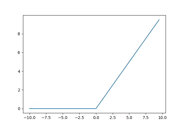
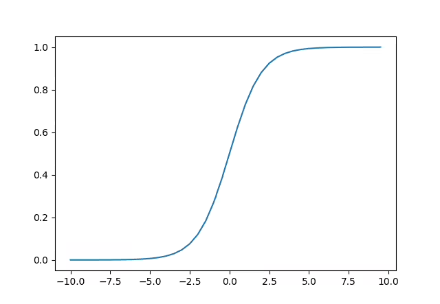
where $\sigma$ is any nonlinear activation function, such as e.g. ReLU or the Sigmoid function.

The shape of $a_1$ is the same as the shape of $z_1$, namely $[m \times h_1]$. For our last layer $O$, we repeat the process:

where $a_2$ has the shape $[m \times o]$.

Let’s code out what we have learned about so far. I assume that you have already a bit of Python experience and that you have Numpy already installed. First, let’s import Numpy and define the architecture of our NN.

import numpy as np

# To ensure reproducibility
random_seed = 42
np.random.seed(random_seed)

neural_network = [
    {'in': 784, 'out': 16, 'activation': 'relu'},
    {'in': 16, 'out': 10, 'activation': 'sigmoid'}
]

Our network has 784 input neurons, which might confuse you. Rightfully so, because we haven’t talked about our data yet. We will be training our NN on the MNIST dataset, which contains handwritten single digits. Let’s write a method, which will download and preprocess the data. For that we need a different library called sklearn. The point of this exercise is to learn about neural networks and not necessarily about data processing. Hence, we can leverage existing libraries that take care of that process such that we can focus on NNs instead.

from sklearn.model_selection import train_test_split
from sklearn.datasets import fetch_openml
from sklearn.preprocessing import MinMaxScaler, OneHotEncoder
from joblib import Memory

def get_mnist(batch_size=64, random_seed=42):
    def split_into_batches(x, batch_size):
        n_batches = len(x) / batch_size
        x = np.array_split(x, n_batches)
        return np.array(x, dtype=object)

    # To cache the downloaded data
    memory = Memory("./mnist")
    fetch_openml_cached = memory.cache(fetch_openml)
    mnist = fetch_openml_cached("mnist_784")

    # Split the data into training and validation sets
    X_train, X_test, y_train, y_test = train_test_split(
        mnist.data, mnist.target, test_size=0.33, random_state=random_seed
    )

    # Normalizes the data
    min_max_scaler = MinMaxScaler()

    # One-Hot encodes the targets
    one_hot_encoder = OneHotEncoder()

    # Split the training data into batches
    X_train = split_into_batches(
        min_max_scaler.fit_transform(np.array(X_train)), batch_size
    )

    #
    X_test = split_into_batches(
        min_max_scaler.fit_transform(np.array(X_test)), batch_size
    )

    # Turn the targets into Numpy arrays and flatten the array
    y_train = np.array(y_train).reshape(-1, 1)
    y_test = np.array(y_test).reshape(-1, 1)

    # One-Hot encode the training data and split it into batches (same as with the training data)
    one_hot_encoder.fit(y_train)
    y_train = one_hot_encoder.transform(y_train).toarray()
    y_train = split_into_batches(np.array(y_train), batch_size)

    one_hot_encoder.fit(y_test)
    y_test = one_hot_encoder.transform(y_test).toarray()
    y_test = split_into_batches(np.array(y_test), batch_size)

    return X_train, y_train, X_test, y_test


X_train, y_train, X_test, y_test = get_mnist()

There is a lot going on in that function. First, we download the data and cache it, such that in subsequent test runs, we don’t have to download the data again every time. Then we perform a train_test_split, which splits the whole data into 2 chunks; in our case ~66.67% of data becomes training data and the remaining ~33% become validation data. The difference between these two is that our NN only uses the training data for learning and the validation data is kept hidden from it. We hide it because we want to test the ability of the NN to generalise to new, never-seen before data. If the NN already saw the validation data during training it would effectively memorise the data and not generalise.

Next, we normalise the data, because as it was in its raw state, the values ranged from [0, 255], which is the “darkness” of a pixel. The higher the value, the darker the pixel. We normalise the data into the range of [0, 1]. No information is lost here, it’s just that NNs tend to be unstable when large numbers are involved. You can test that yourself by not performing the normalisation step and see what happens!

Now that we have the data ready, let’s actually have a look at what’s inside. Each handwritten digit is a 28x28 image; hence our NN has 784 input nodes. Here’s an example of what these digits look like

import matplotlib.pyplot as plt

X_train, y_train, X_test, y_test = get_mnist()
# Get from the first batch the first example and shape it back to its original form of 28x28 pixels
example = X_train[0][0].reshape(28, 28)
# Get the corresponding target value. Since its a one hot encoded array, we use argmax.
example_target = np.argmax(y_train[0][0])

plt.imshow(example)
plt.title(f"It's a {example_target}!")
plt.show()

And we are going to build a NN which will be able to identify these numbers just by looking at their pixel values. Perhaps you are a little confused as to what “one-hot encoding” means. Initially, the data was a 28x28 pixel image and the target was a simple string, e.g. “3”. In the end we want to have a probability estimate from the NN, e.g. how confident is the NN that the given number is a 3. Therefore we map all possible classes to an array and set one value in the array to 1 (hence the name, one element in the array is “hot”).

Doing that makes sense. If the given number is a 3 and we make the target look like this [0 0 0 1 0 0 0 0 0 0] then we essentially tell the NN to be as confident as possible that this particular example is a 3. Hopefully, that was understandable (and if not, you can shoot me a mail or raise an issue in GitHub).

In the previous section we defined the architecture of our NN and prepared our data. Now, we need to actually create the weights and biases of our NN. To do that, we need to iterate over our architecture dictionary and initialize the weight and bias matrices.

def initialise_weights_and_biases(nn_architecture):
    parameters = {}
    for idx, layer in enumerate(nn_architecture):
        n_input = layer["in"]
        n_output = layer["out"]

        parameters[f"weights {idx}->{idx+1}"] = np.random.randn(n_input, n_output) * 0.1
        parameters[f"bias {idx+1}"] = (
            np.random.randn(
                n_output,
            )
            * 0.1
        )

    return parameters

Notice how the shape of the bias is initialised as np.random.randn(n_output,)* 0.1 as we mentioned earlier. This is done so that Numpy can later perform broadcasting. In the NN architecture we had also defined the activation functions, so let’s also code them out.

def sigmoid(Z):
    return 1 / (1 + np.exp(-Z))


def relu(Z):
    return np.maximum(0, Z)

With this, everything should be ready for coding out the forward propagation of the NN.

Before we start coding the forward propagation step, let’s first visualise where we are so far. We have 1 NN consisting of 3 layers: the input, hidden and output layer. The input layer has 784 nodes, the hidden layer has 16 nodes and the output layer has 10 nodes. Then, we also have 2 sets of weights and biases (W&B): the W&Bs between the input and hidden layer and between the hidden and output layer.

Let’s think for a moment what we would really need to compute for forward propagation. In essence, we only need to compute $a_i \forall i = 0, 1, 2$ (this is spoken as ”$a_i$ for all $i$ equals $0, 1, 2$”, or in other words $a_0, a_1, a_2$).We already know $a_0$, which is simply our training data $X$. Therefore, when we loop over our NN architecture, we can skip the first index and simply start at $1$. But that comes later. For now, let’s define the forward propagation for a single layer $i$. That would be

In Python code that would be:

def forward_single_layer(a_prev, w, b, activation_function):
    z = a_prev @ w + b
    a = activation_function(z)

    return a, z

Now that we have written the code for a single layer, we need to write a loop, which iterates over our NN architecture and applies this single layer propagation to every layer. Let’s define the forward method for that.

def forward(x, nn_parameters, nn_architecture):
    # If our network has 3 layers, our dictionary has only 2 entries.
    # Therefore we need to add 1 on top
    n_layers = len(nn_architecture) + 1
    # The memory is needed later for backpropagation
    memory = {}
    a = x

    # We have 3 layers, 0, 1 and 2 and want to skip 0
    # Therefore we start at 1
    for i in range(1, n_layers):
        a_prev = a
        activation_function = globals()[nn_architecture[i - 1]["activation"]]
        w = nn_parameters[f"weights {i-1}->{i}"]
        b = nn_parameters[f"bias {i}"]

        a, z = forward_single_layer(a_prev, w, b, activation_function)

        memory[f"a_{i - 1}"] = a_prev
        memory[f"z_{i}"] = z

    return a, memory

Let’s try out our NN, which has not been trained yet, to see what it thinks the first number is (hint: it’s the “3” that we saw earlier).

neural_network = [
    {"in": 784, "out": 16, "activation": "relu"},
    {"in": 16, "out": 10, "activation": "sigmoid"},
]
X_train, y_train, X_test, y_test = get_mnist()
parameters = initialise_weights_and_biases(neural_network)

a, memory = forward(X_train[0][0].reshape(1, 784), parameters, neural_network)
print(f"I'm {np.round(np.max(a) * 100, 2)}% sure that it's a {np.argmax(a)}.")
print(f"The number was a {np.argmax(y_train[0][0])}")

It seems our NN was fairly confident that it was a 6, but unfortunately, it was a 3. Now that we have the forward propagation figured out and have written the code for it, it’s time to tackle the actual difficult part in NN: backpropagation!

In backpropagation (BP) we calculate the error, i.e. the difference between what our NN outputs and what’s actually the desired output and then send that error back through the NN to adjust its W&B. For now, let’s focus on BP for a single layer before we apply it to the whole network. We can once again derive the formula for BP by noting what we actually want to compute. We want to calculate the gradients of the weights and biases of our NN. But as someone once said to a pair of shoes: what are those? To understand what a gradient is we need to take a little detour. If you know what a gradient is, you can skip that part.

Detour: Gradients

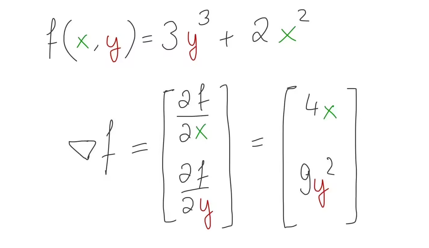
First I want you to calculate the derivative of $f(x) = 2x^2$. No problem, right? Obviously, it’s $f(x)' = 4x$.Now I want you to calculate the derivative of $f(x, y) = 3y^3 + 2x^2$. At this point you might be confused. The derivative with respect to what variable? A good question. The point is you can only take derivatives w.r.t. a single variable, e.g. $x$ or $y$ in our example. But what if you wanted all the derivatives?

That’s where gradients come in. A gradient is a vector which contains all the (first) derivatives w.r.t. every variable. In our example, the gradient would be:

But why would we ever want to compute these? Gradients have the property that they point in the direction of steepest ascend. Take a derivative for example.

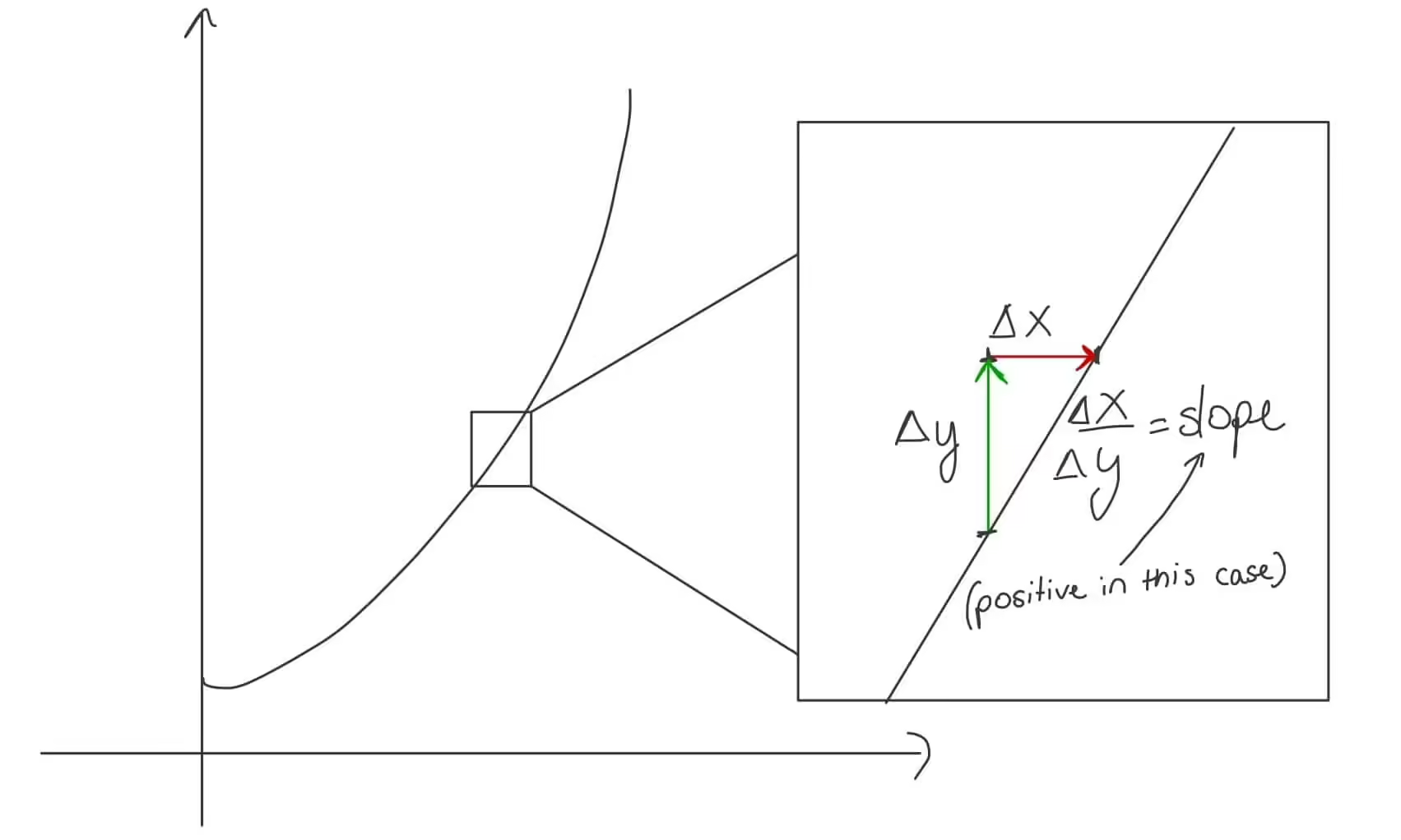
A derivative - in a sense - also points in the direction of steepest ascend but that concept makes little sense in the context of a line, since there is only one direction the line goes. If you wanted to perform gradient descent on this function $f(x) = 2x^2$ to find the value of $x$ which minimises $f$, how would you do it? We know that the gradient (i.e. derivative in the case of only one variable) points in the direction of steepest ascend. If we compute the gradient of $f$ and add that to $x$ then we would increase $f$, which is not what we want. We want $f$ to be as small as possible. Therefore, we subtract from $x$ the gradient of $f$.

The same will be done later in our NN, only that $f$ will be the cost function and the gradient contains significantly more entries. But don’t fret. It’s actually quite simple. Now that you know what a gradient is, we can continue on our quest to understand BP.

We mentioned before that we want to calculate the gradients of the weights and biases in our NN but how can that be done? For that we have to simplify things to a NN, that has only a single input neuron, weight, bias and output neuron.

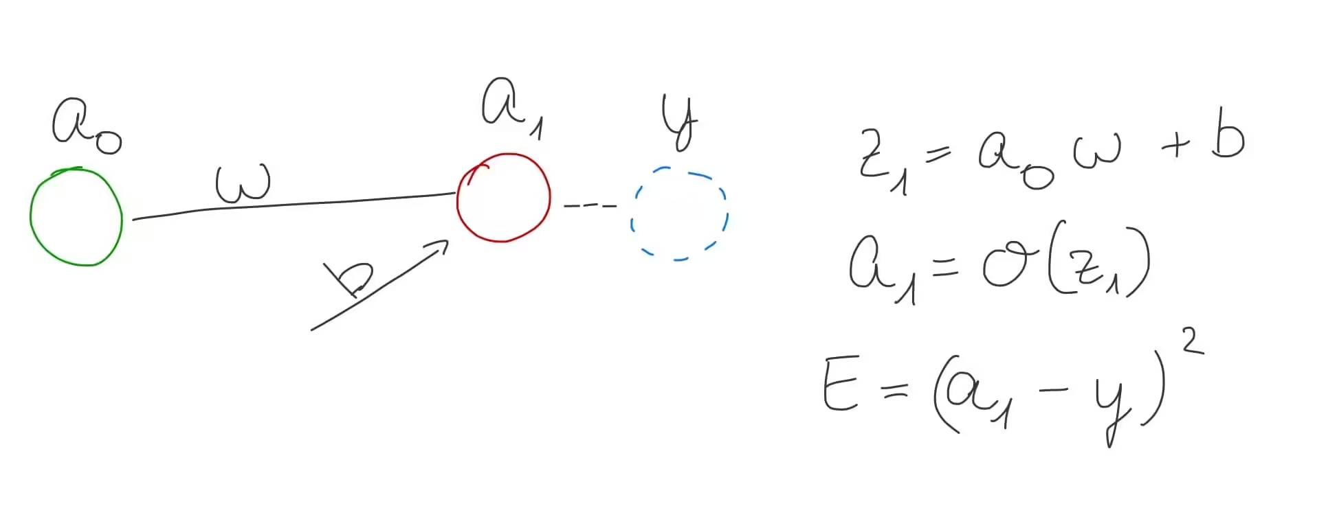
In the example above, we use the mean squared error. To calculate the gradient $dW$ we need to use the chain rule. Using the chain rule we can ask how does a little change to $w$ change the error $E$?

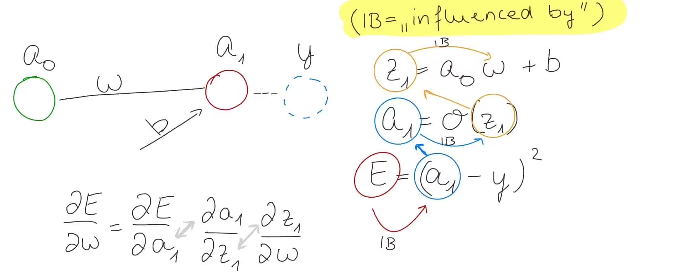
In case you are not familiar with the chain rule, I would highly advise to go and refresh your knowledge with some YouTube videos on the matter. There are a lot of truly helpful videos that can teach you the essence of the chain rule. Personally, I visualise the chain using the equations. In fact, in the image above, you can kind of see the chain. If you want to know how $\frac{d}{dw}$ changes w.r.t. $w$ (which is a couple of equations away) you have to “find the path” to $w$. In this case you first go to $a_1$ then from $a_1$ to $z_1$ and then finally from $z_1$ to $w$. And for each “hop” from $w \to b$ means calculating the partial derivative of a w.r.t. b.

Luckily, in our case, the partial derivatives are easy to calculate. I will leave it to you to calculate the partial derivative w.r.t. the bias.

But this is sort of a special case. What do we need for the “general case”, i.e. something we could run in a loop. While the middle and right equations above look the same for every layer, the left-most one doesn’t.

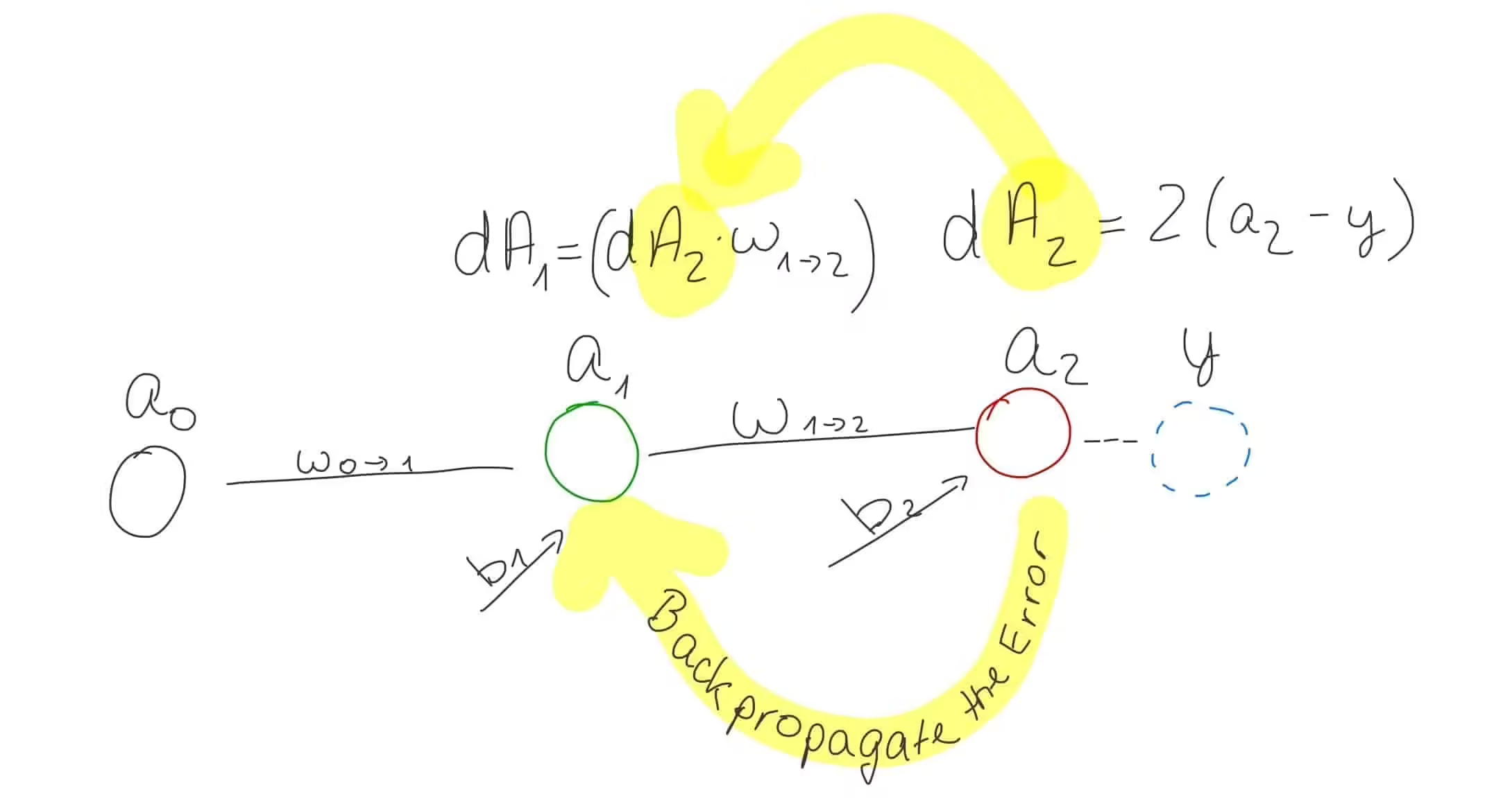
In a way, we took the error from the last layer and have sent it back one layer. Note that we need to weight the error by the weights. And with that we have the ingredients to define BP for a single, generic layer.

The last thing required is to ensure that we have our dimensionalities right. Take a look at this again:

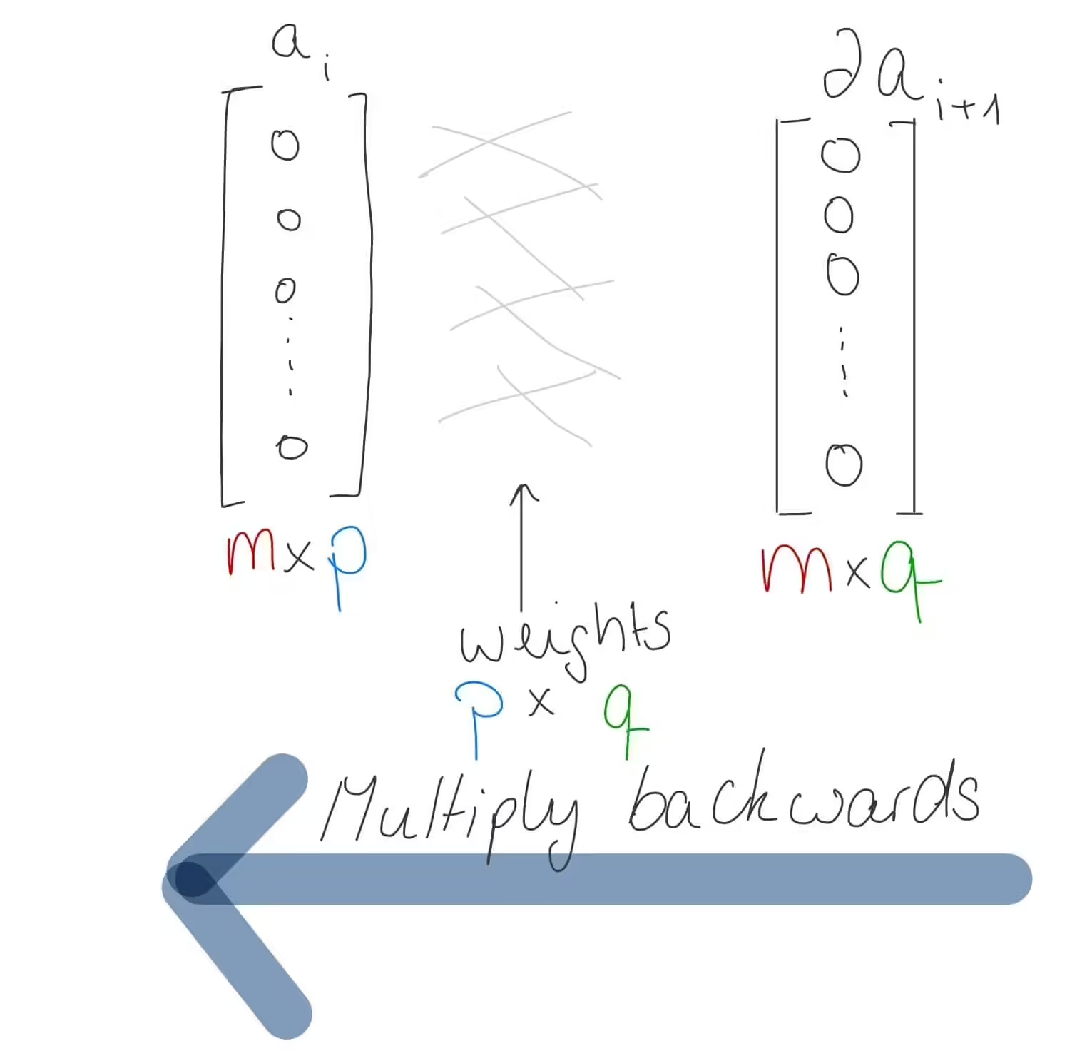
To multiply the delta of the next layer with the weights, we need to transpose the weight matrix, such that the dimensions of our matrices fit.

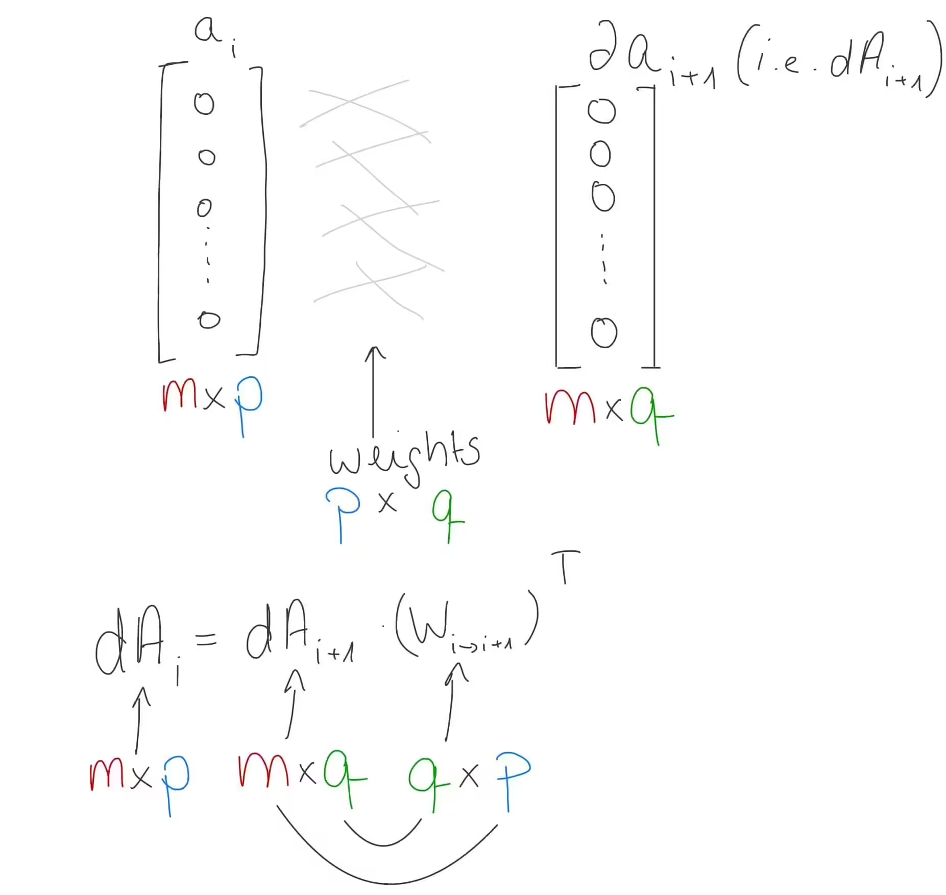
Now that we know the math of BP for a single layer, it’s time to write that out in Python.

def backpropagation_single_layer(dA, w, z, a_prev, activation_function):
    m = a_prev.shape[0]
    backprop_activation = globals()[f"{activation_function}_backward"]

    delta = backprop_activation(dA, z)
    dW = (a_prev.T @ delta) / m
    dB = np.sum(delta, axis=1, keepdims=True) / m
    dA_prev = delta @ w.T

    return dW, dB, dA_prev

We also need the derivatives of our activation functions. I’ll save some time by skipping their derivations, since there are several activation functions and the derivations of their derivatives don’t really add anything to the understanding of a NN. Just know that you need the derivative of these activation functions.

def sigmoid_backward(dA, Z):
    sig = sigmoid(Z)
    return dA * sig * (1 - sig)


def relu_backward(dA, Z):
    dZ = np.array(dA, copy=True)
    dZ[Z <= 0] = 0
    return dZ

Now that we have defined BP for a single layer, it’s time to put that in a loop and to iterate over all our layers.

def backward(target, prediction, memory, param_values, nn_architecture):
    gradients = {}
    dA_prev = 2 * (prediction - target)
    # If our network has 3 layers, our dictionary has only 2 entries.
    # Therefore we need to add 1 on top
    n_layers = len(nn_architecture) + 1

    # Loop backwards
    for i in reversed(range(1, n_layers)):
        dA = dA_prev

        # Memory from the forward propagation step
        a_prev = memory[f"a_{i-1}"]
        z = memory[f"z_{i}"]

        w = param_values[f"weights {i-1}->{i}"]

        dW, dB, dA_prev = backpropagation_single_layer(
            dA, w, z, a_prev, nn_architecture[i - 1]["activation"]
        )

        gradients[f"dW_{i-1}->{i}"] = dW
        gradients[f"dB_{i}"] = dB

    return gradients

With that, the last step is to update our weights and biases. Remember: if we add the gradient (which is the direction of steepest ascend) we would increase the error. Therefore, we need to subtract the gradients. But not the whole gradient though. We multiply the gradient with a learning rate $\alpha=0.1$ to make the changes in our NN not so abrupt and rather slow and steady.

def update(param_values, gradients, nn_architecture, learning_rate):
    n_layers = len(nn_architecture) + 1
    for i in range(1, n_layers):
        param_values[f"weights {i-1}->{i}"] -= (
            learning_rate * gradients[f"dW_{i-1}->{i}"]
        )
        param_values[f"bias {i}"] -= learning_rate * gradients[f"dB_{i}"].mean()
    return param_values

The code is almost finished. All that’s left is to verify that everything works. For that, the validation data will come into play. Let’s write some code that gives us the current accuracy of our NN.

def get_current_accuracy(param_values, nn_architecture, X_test, y_test):
    correct = 0
    total_counter = 0
    for x, y in zip(X_test, y_test):
        a, _ = forward(x, param_values, nn_architecture)
        pred = np.argmax(a, axis=1, keepdims=True)
        y = np.argmax(y, axis=1, keepdims=True)
        correct += (pred == y).sum()
        total_counter += len(x)
    accuracy = correct / total_counter
    return accuracy

And now, let’s write our final training loop to see how well we are performing.

def main():
    neural_network = [
        {"in": 784, "out": 16, "activation": "relu"},
        {"in": 16, "out": 10, "activation": "sigmoid"},
    ]
    X_train, y_train, X_test, y_test = get_mnist()
    parameters = initialise_weights_and_biases(neural_network)

    n_epochs = 50
    learning_rate = 0.1
    for epoch in range(n_epochs):
        for x, y in zip(X_train, y_train):
            a, memory = forward(x, parameters, neural_network)
            grads = backward(y, a, memory, parameters, neural_network)
            update(parameters, grads, neural_network, learning_rate)
        accuracy = get_current_accuracy(parameters, neural_network, X_test, y_test)
        print(f"Epoch {epoch} Accuracy = {np.round(accuracy, 4) * 100}%")

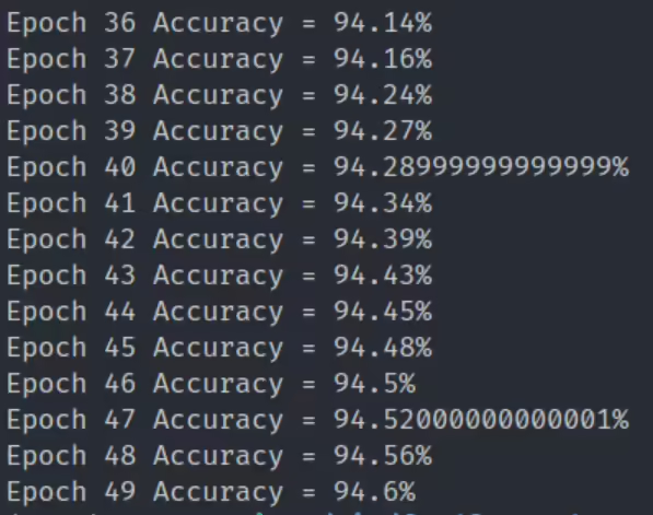
And here’s the final performance of our little network. Impressively, it managed to get an accuracy of over 94% with just a single hidden layer. You can play around with the code to add more layers to see if you can improve the performance.

That’s it! We coded a neural network with nothing but our bare hands. Here’s the code of this project.

Thanks a lot for reading this post and I will see you in the next one!