Proximal Policy Optimization

2024-01-02

Contents

• Introduction
• Lightning FAQ
• Back to PPO

Introduction

Proximal Policy Optimization (PPO) is one of the most successful RL algorithms out there. It is known for its ease of tuning and excellent performance. Today, we will cover PPO and you will see how to implement it yourself using Jax! So, let’s get started!

First, where does PPO fall into the RL algorithm buckets? PPO is an Actor-Critic algorithm, which means it falls into the policy gradient faction. In fact, it’s a natural extension to the vanilla policy gradient algorithm as we will see in a moment. First, let’s review the vanilla policy gradient algorithm (which we had already covered in this blogpost before).

First, we define the reward (infinite horizon and discounted) given some trajectory

Next, what is the probability to sample that particular trajectory? We define it as

Spoken out loud, the above equation translates to the probability to sample a particular trajectory $\tau$ given a policy $\pi$ with parameters $\theta$ is equal to the the probability of the initial state times the product of the probability to land in a state $s_{t+1}$ given the current state $s_t$ and the action $a_t$ times the probability to pick the action $a_t$ given the current state $s_t$ .

Now that we now the probability to sample a trajectory given our current policy, we define the objective function as

Given that objective function, we next computed the gradient of the objective function. I won’t go into the details here, but if you want to understand the details, I suggest you read my other blog post. Anyway, the gradient of the objective function is defined as

Furthermore, we had also improved this objective function by including a baseline in the form of a value network, like so:

With this gradient, we can update the parameters of our policy, which in turn should increase our rewards. In the update function, we had also included a learning rate αα to make our step sizes not so big (to avoid overshooting). But what is the biggest possible step we can take in our gradient update while still keeping the training stable? That’s the question that PPO tries to answer.

One problem vanilla policy gradients have is that the performance of the agent increases over time (which in of itself is a good thing) but then - at some point - dramatically crashes and never recovers. That often leads to a reward curve like this:

Reward Curve

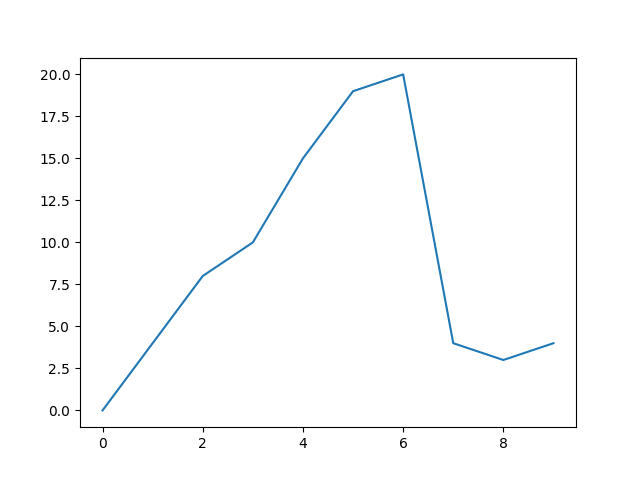
This is very frustrating! Your agent was so close to perfection and then it plummets into the abyss forever. What a tragedy :( We want to add some constraints to ensure that our agent doesn’t experience this kind of catastrophic forgetting.

Let’s change the objective function a bit and remove the total trajectory return $R(\tau)$ from the equation. Instead, we will use the advantage function $A(s_t,a_t)$. The advantage function gives us a measure of how good taking some action $a_t$ at state $s_t$ was compared to the expected return. More specifically, one way of defining it is

In other words, it’s the difference between taking action $a_t$ at state $s_t$ and then following the policy and the value of being in state $s_t$. If you subtract these two, you get left with the value of performing action $a_t$.

Note, that there are other ways to calculate the advantage function (and we will learn about one of them later). Also note that $Q$ and $V$ are themselves expectations and what we are comparing are expected values.

Now, changing our objective function to include the advantage function, we get

But why do we bother with the advantage function at all? Can’t we just use the return of the trajectory $R(\tau)$ as we had before? Of course, we could, but the problem with it is that it as a lot of variance. Consider the following example in which your agent gets these rewards:

5, 0, -5, 10, 0, -5, -5

The sum of these rewards is 0, i.e. $R(\tau) = 0$. This gives us very little information about what actions lead to which results. We have to look at each action within the trajectory (kind of like zooming into the trajectory) to get more information out of it.

The advantage function also gives us another, very useful hint. It’s sign tells us if we should pursue that action again in the future. If it’s positive, then the performed action has given as more reward than expected. Remember, the advantage is the difference between $Q(s, a)$ and $V(s)$. If it was 0, then the performed action at that state and the value of that state were equal, i.e. exactly as expected. If it was negative, it would mean that on average the agent was better off with any other action. Vice versa, a positive advantage tells us that the performed action was better than expected.

Let’s put this information safely away in a drawer in our brain and come back to PPO and the problem it’s trying to solve, which was mitigating catastrophic forgetting. At some point - in vanilla policy gradients - an update happens which shouldn’t have happened. PPO tries to avoid this by making smaller updates.

The way PPO does is this by clipping the probability ratio within the objective function into a certain range, which is the hyperparameter $\epsilon$. It is defined as

where $A(·)$ is just a shortform for $A(s_t, a_t)$. We will talk about what the probability ratio means.

Lightning FAQ

The vanilla objective function (not the gradient, just the objective function) was defined as

$J(\pi_\theta) = \mathbb{E}_{\tau \sim \pi_\theta} R(\tau) = \int P(\tau|\pi_\theta)R(\tau)$

but why did we bother deriving the gradient at all? Don’t we have fancy autograd packages which do all that for us?

The answer is that - yes, we do have amazing autograd packages but even they can’t changes the laws of the universe. The issue - namely why we couldn’t just let the autograd rip and do everything for us - was that we didn’t have $P(\tau|\pi_\theta)$ because that depends on the dynamics of the environment - something we don’t have. That’s the whole reason, we have to do all that math to get this into a differentiable form.

Luckily, that issue is not present in the PPO objective function, which means we don’t have to derive it by hand. That’s because everything in the function is either something we have or can easily compute. Nice! Quick FAQ over!

Back to PPO

Let’s talk about the components of the objective function and we will cover the easy things first. As mentioned before, $\epsilon$ is a hyperparameter, which is between 0 and 1. The min function is hopefully something I don’t have to explain. The clip function does exactly what numpy.clip does. Next up is the ratio $r_\theta(t)$, something a bit more interesting.

Mathematically, the ratio is defined as “the ratio of probabilities between your current policy and the previous policy”, i.e.

Let’s stop and think for a moment what this ratio tells us by interpreting it. If the action probability in the current policy is higher than in the previous iteration (i.e. the action is now more likely than before), then the ratio will be positive. If the advantage function is now also positive, then the whole thing becomes positive, which will encourage the action even more in the future. And vice versa.

This ratio is like a scaling factor, i.e. it weighs the advantage function. We constrain the ratio in the range of $1 \pm \epsilon$ (that’s how much the ratio is clipped by). We do this clipping, to prevent a too-large update, e.g. if the advantage for some reason just explodes in the positive direction, which would add a lot of variance and, thus, destabilise the training process.

In essence, the ratio tells us how likely a probability is now compared to before. It becomes more likely if the action lead to a positive advantage. A positive advantage is achieved if the action performed better than expected by our baseline (and vice versa).

One side note here: when we are referring to the policy $\pi(a_t|s_t)$, we talk about a probability distribution of taking action $a_t$ at state $s_t$. The authors in the PPO paper defined the ratio the same way we did earlier. In practice when we implement this, we use log probabilities. We use logs here because probabilities can get very small and our networks don’t learn so effectively when very small numbers are involved. When you log everything, those small numbers get larger, which introduce numerical stability. So, when you implement this objective function, then in my opinion, the authors could have written it like this:

where $\pi(·)$ stands for $\pi(a_t|s_t)$. Note, that this is 100% equivalent mathematically to simply computing the ratios directly. But in using logs, we introduce more stability. Unfortunately, these details don’t often make it into the paper - much to my disappointment, because these kind of notes are incredibly valuable to beginners in the field.

Before we take a look into the advantages, let’s quickly implement what we talked about so far. As it turns out, the implementation is quite simple and I will refer you to this implementation from the rlax library.

def clipped_surrogate_pg_loss(
    prob_ratios_t: Array,
    adv_t: Array,
    epsilon: Scalar,
    use_stop_gradient=True) -> Array:
  """Computes the clipped surrogate policy gradient loss.

  L_clipₜ(θ) = - min(rₜ(θ)Âₜ, clip(rₜ(θ), 1-ε, 1+ε)Âₜ)

  Where rₜ(θ) = π_θ(aₜ| sₜ) / π_θ_old(aₜ| sₜ) and Âₜ are the advantages.

  See Proximal Policy Optimization Algorithms, Schulman et al.:
  https://arxiv.org/abs/1707.06347

  Args:
    prob_ratios_t: Ratio of action probabilities for actions a_t:
        rₜ(θ) = π_θ(aₜ| sₜ) / π_θ_old(aₜ| sₜ)
    adv_t: the observed or estimated advantages from executing actions a_t.
    epsilon: Scalar value corresponding to how much to clip the objecctive.
    use_stop_gradient: bool indicating whether or not to apply stop gradient to
      advantages.

  Returns:
    Loss whose gradient corresponds to a clipped surrogate policy gradient
        update.
  """
  chex.assert_rank([prob_ratios_t, adv_t], [1, 1])
  chex.assert_type([prob_ratios_t, adv_t], [float, float])

  adv_t = jax.lax.select(use_stop_gradient, jax.lax.stop_gradient(adv_t), adv_t)
  clipped_ratios_t = jnp.clip(prob_ratios_t, 1. - epsilon, 1. + epsilon)
  clipped_objective = jnp.fmin(prob_ratios_t * adv_t, clipped_ratios_t * adv_t)
  return -jnp.mean(clipped_objective)

At the end, we return the negative mean. We do this, because we want to maximise the objective function (as opposed to minimising a loss function as is normally done in ML). That’s why we return the negative mean.

But as you can see in that function, we need to pass in the advantages $A_t(s_t,a_t)$, which means we need an array of these advantages with the shape n_timesteps.

Now, let’s see how we can implement the advantage function. I mentioned before that one way to implement it would be to find the difference between $Q$ and $V$, but we don’t want another 2 networks to keep track of those. Instead, we can compute the General Advantage Estimation or GAE.

The GAE is defined as

where $\delta_{t+l}$ is the TD error at time $t+l$ and $\lambda$ is a hyperparameter between 0 and 1 and the $\gamma$ is the discount factor. The TD error is defined as

Usually, we don’t really deal with infinite horizons, so we can rewrite the advantage function as

The parameters $\gamma$ and $\lambda$ are numbers between 0 and 1 and are hyperparameters. As you know, $\gamma$ is the discount factor and $\lambda$ allows you to interpolate between TD(0) (which is $\lambda=0$) and Monte Carlo estimates (which would correspond to $\lambda=1$).

Luckily, DeepMind’s rlax library has this also implemented, see here for their implementation.

def truncated_generalized_advantage_estimation(
    r_t: Array,
    discount_t: Array,
    lambda_: Union[Array, Scalar],
    values: Array,
    stop_target_gradients: bool = False,
) -> Array:
  """Computes truncated generalized advantage estimates for a sequence length k.

  The advantages are computed in a backwards fashion according to the equation:
  Âₜ = δₜ + (γλ) * δₜ₊₁ + ... + ... + (γλ)ᵏ⁻ᵗ⁺¹ * δₖ₋₁
  where δₜ = rₜ₊₁ + γₜ₊₁ * v(sₜ₊₁) - v(sₜ).

  See Proximal Policy Optimization Algorithms, Schulman et al.:
  https://arxiv.org/abs/1707.06347

  Note: This paper uses a different notation than the RLax standard
  convention that follows Sutton & Barto. We use rₜ₊₁ to denote the reward
  received after acting in state sₜ, while the PPO paper uses rₜ.

  Args:
    r_t: Sequence of rewards at times [1, k]
    discount_t: Sequence of discounts at times [1, k]
    lambda_: Mixing parameter; a scalar or sequence of lambda_t at times [1, k]
    values: Sequence of values under π at times [0, k]
    stop_target_gradients: bool indicating whether or not to apply stop gradient
      to targets.

  Returns:
    Multistep truncated generalized advantage estimation at times [0, k-1].
  """
  chex.assert_rank([r_t, values, discount_t], 1)
  chex.assert_type([r_t, values, discount_t], float)
  lambda_ = jnp.ones_like(discount_t) * lambda_  # If scalar, make into vector.

  delta_t = r_t + discount_t * values[1:] - values[:-1]

  # Iterate backwards to calculate advantages.
  def _body(acc, xs):
    deltas, discounts, lambda_ = xs
    acc = deltas + discounts * lambda_ * acc
    return acc, acc

  _, advantage_t = jax.lax.scan(
      _body, 0.0, (delta_t, discount_t, lambda_), reverse=True)

  return jax.lax.select(stop_target_gradients,
                        jax.lax.stop_gradient(advantage_t),
                        advantage_t)

It uses a slightly different notation, namely that they truncate the episode at timestep $k$ whereas in our formula above, we didn’t truncate the episode and instead let it run until the terminal step $T$.

As another side note, if you look closely at the advantage function, you will notice the value function $V(s_t)$. This indicates that we need another neural network to keep track of the value function. This also means, that we have an actor-critic architecture.

Now, we have all the ingredients to implement PPO. We have the objective function, the advantage function and the ratio. Let’s implement all this first for CartPole and then for a more complex environment such as LunarLander.