REINFORCE - Policy Gradient

2023-11-19

Contents

• Introduction
• The Objective Function
• Writing Some Code

Introduction

Before we dive deep into the REINFORCE algorithm, I highly suggest you first read the basics of RL before continuing. This post will assume that you have a basic understand of the concepts introduced in the basics of RL post. Some parts will be repeated here for completeness, but it is highly recommended to read the basics of RL post first.

The Objective Function

We know that there are two ways to define the return from a trajectory:

• finite horizon undiscounted return

• infinite horizon discounted return

And we also know that the probability to “sample” a trajectory depends on the current policy and is defined as

With that in mind, we can define the objective function as the expected return, in other words:

Here’s a helpful hint: think of gradients as an operation, like plus or minus. In the case of plus or minus, the operation is denoted as + or - but for the gradient, we denote that as $\nabla_x$ , where $x$ is the parameter we want to take the gradient with respect to. In our case, it’s $\theta$ . So, if we take the gradient of the objective function like so:

$\nabla_\theta (J(\pi_\theta))$

we get a vector which points in the direction of steepest ascend.

We actually don’t need the paranthesis around $J$; it’s just there to emphasise that the gradient operator applies only to the next term. Since there is only a single term, the paranthesis are redundant.

Let’s understand the gradient a bit better and use a simple example function like

In RL notation, we usually just write $\pi_\theta$ as a shortform for $\pi_{\theta_0,\theta_1,..,\theta_n}$ where each $\theta_i$ is a parameter in the model (i.e. the neural network).

When we compute the gradient of $f$ with respect to the parameters $\theta$, we get a vector as result! You might be wondering why the result is a vector. Think of it this way: for you, it should be no problem to compute the derivative of the function $f$ w.r.t. $\theta_0$ or w.r.t. $\theta_1$ individually. In fact, the results of both derivates are

A gradient simply computes all derivates w.r.t. every parameter at the same time. That’s why you get a vector: it’s because the function has multiple parameters and you need a vector that’s as long as the number of parameters of your function (in our simple example, that would be 2). So, the gradient is:

$\nabla_{\theta}f = \begin{bmatrix} \frac{\partial f}{\partial \theta_0} \\ \frac{\partial f}{\partial \theta_1} \end{bmatrix}$

Now you have a vector which has the same size as the parameters. This gradient points to the direction of steepest ascend, which means that if you add this vector to $\theta$, then the underlying function $f$ will increase! Similarly, if you subtract the gradient, the underlying function will decrease. That’s why - in the context of machine learning - people talk about gradient descent. You take the gradient of the loss function and subtract it from your parameters, because you want to make the loss smaller. In our case, it’s reverted because we have an objective function which we want to make as big as possible (because that means we got more reward). This also means, that we take the gradient and add it to our parameters as that makes $J$ bigger.

So back to RL, we want to find the gradient of $J$ so that we can add the gradient vector to our parameters $\theta$ to get more reward:

Here, $\alpha$ is the learning rate and $\nabla_{\theta}J(\pi_{\theta})|_{\theta_k}$ refers to the gradient w.r.t. $\theta_k$ where $k$ is the current iteration. Simply put, take the current parameters, add the gradient on top, and voilá, you got the next set of parameters.

Alright, let’s get started with the policy gradient. These steps will be a bit more mathematically heavy, so buckle up! I’ll try to explain each step along the way.

The Gradient

Expand Expectation

Move Gradient into the Integral

Everything up until now should have been very easy. Now we get to one of the more tricky parts. We need to perform the so-called log-derivative trick. We do that because computing the gradient of the probability directly is very complex and also because logs introduce a lot of numerical stability, especially as numbers get smaller.

The log-derivative trick is quite simple: the derivative of $\log x$ is $\frac{1}{x}$ . So we start with $\log P(\tau|\theta)$ and want to compute the gradient w.r.t. $\theta$ .

Apply the Gradient & the Chain Rule

Differentiating the Outer Function (Logarithm)

Diff. the Inner Function

Multiplying the Derivatives as per Chain Rule

Chain Rule Result

Rearranging to Isolate $\nabla_{\theta}P(\tau|\theta)$

Multiply the probabilities on both sides

Cancel Stuff out

Alright, now you know about the log-derivative trick. Let’s go back to the gradient of the objective function. We had just brought in the gradient into the integral.

(Reminder) Move Gradient into the Integral

Put in the Result from the Log-Derivative Trick

Back to Expectation

Now it’s time to have a closer look at this term $\nabla_{\theta}\log P(\tau|\theta)$. First, applying the log, we get

Simple stuff so far: just apply the log to every term in the equation. Next, we apply the gradient operation to each term (because the derivative of a sum is the sum of the derivatives). We get:

In this equation, each term which has nothing to do with $\theta$ becomes $0$ . Removing those, we get:

(Reminder) Back To Expectation

Replacing $\nabla_\theta \log P(\tau|\theta)$

Now that we have this form, and since this is an expectation - we can sample trajectories from our environment to estimate the policy gradient. The next question is: how can we actually implement this?

Remember, how I mentioned that taking the gradient is like an operation? This means, all we need is to implement

in a Python function and then compute the gradient of that function by using something like grad(objective_function)(params). Conveniently, most neural network frameworks have this functionality built-in. For example, in PyTorch, you can simply call loss.backward() and it will compute the gradient for you. In JAX, it’s even more convenient as you can simply call jax.grad(objective_function) and it will return the gradient function for you.

Writing Some Code

Alright, now it’s time to actually write some code. Let’s start simply by implementing our policy neural network first. In this blog post, I’m using Equinox, which is a neural network library built on top of JAX, but the code can easily be translated into any other machine learning framework.

import equinox as eqx
import jax
import jax.numpy as jnp
from icecream import ic
from jaxtyping import Array, Float32, PRNGKeyArray, PyTree


class Policy(eqx.Module):
    """Policy network for the policy gradient algorithm in a discrete action space."""

    mlp: eqx.nn.MLP

    def __init__(self, in_size: int, out_size: int, key: PRNGKeyArray) -> None:
        key, *subkeys = jax.random.split(key, 5)
        self.mlp = eqx.nn.MLP(
            in_size=in_size, out_size=out_size, width_size=32, depth=2, key=key
        )

    def __call__(self, x: Float32[Array, "state_dims"]) -> Array:
        """Forward pass of the policy network.
        Args:
            x: The input to the policy network.
        Returns:
            The output of the policy network.
        """
        return self.mlp(x)

Our policy is just a simple MLP with a ReLU activation function. The input is the state and the output are the logits for each action. Next up, the objective function:

def objective_fn(
    policy: PyTree,
    states: Float32[Array, "n_steps state_dim"],
    actions: Float32[Array, "n_steps"],
    rewards: Float32[Array, "n_steps"],
):
    logits = eqx.filter_vmap(policy)(states)
    log_probs = jax.nn.log_softmax(logits)
    log_probs_actions = jnp.take_along_axis(
        log_probs, jnp.expand_dims(actions, -1), axis=1
    )
    return -jnp.mean(log_probs_actions * rewards)a
    # alternatively:
    # log_probs_actions = tfp.categorical.Categorical(logits=logits).log_prob(actions)
    # return -tf.reduce_mean(log_probs_actions * rewards)

When we take the gradient of the objective function by calling jax.grad(f), we will arrive at the policy gradient. You might also be wondering why we return the negative mean. When we use optimiser libraries such as optax, those libraries expect to perform gradient descent and not gradient ascent. The reasoning is, that 99% of the time, you want to minimise the loss function and not maximise it. But in our case, we actually want to maximise the objective function, so we have to revert the sign to make it a minimisation problem.

But what we have there is not a real loss function in the traditional sense. There is a beautiful explanation on OpenAI’s Spinning Up tutorials on this topic:

[…] it is common for ML practitioners to interpret a loss function as a useful signal during training—if the loss goes down, all is well.” In policy gradients, this intuition is wrong, and you should only care about average return. The loss function means nothing.

Next, we will need a function to sample trajectories from our environment. For this, we will use the this function, which performs a single rollout of the environment with discrete actions:

class RLDataset(Dataset):
    def __init__(self, states, actions, rewards, dones) -> None:
        self.rewards = torch.tensor(rewards)
        self.actions = torch.tensor(actions)
        self.obs = torch.tensor(states)
        self.dones = torch.tensor(dones)

    def __len__(self) -> int:
        return len(self.rewards)

    def __getitem__(
        self, idx
    ) -> tuple[torch.Tensor, torch.Tensor, torch.Tensor, torch.Tensor]:
        return (
            self.obs[idx],
            self.actions[idx],
            self.rewards[idx],
            self.dones[idx],
        )


def rollout_discrete(
    env: gym.Env, action_fn: Callable, action_fn_kwargs: dict, key: PRNGKeyArray
) -> RLDataset:
    obs, _ = env.reset()

    observations = []
    actions = []
    rewards = []
    dones = []

    while True:
        key, subkey = jax.random.split(key)
        observations.append(obs)

        action = np.array(action_fn(obs, **action_fn_kwargs, key=subkey))
        obs, reward, terminated, truncated, _ = env.step(action)
        done = terminated or truncated
        actions.append(action)
        rewards.append(reward)
        dones.append(done)

        if done:
            break

    dataset = RLDataset(
        np.array(observations), np.array(actions), np.array(rewards), np.array(dones)
    )

    return dataset

    )

The beautiful thing about this function is, that it’s completely agnostic to the environment and the function, which actually selects the action. The other beautiful thing is - and this is JAX exclusive - is that there are implementations of some environment that you can JIT compile, which means you can run the environment on your GPU! This is absolutely amazing! Even better, recently, MuJoCo and Brax announced that they will support JAX natively, which means you can run those environments on your GPU as well! Now, if that’s not cause for celebration, I don’t know what is!

Alright, we have our policy, we have our objective function, and we have a function to sample trajectories from our environment. Now, we need to put it all together and train our policy.

We’ll write a train function like so:

def train(
    policy: PyTree,
    env: gymnasium.Env,
    optimiser: optax.GradientTransformation,
    n_epochs: int = 50,
    n_episodes: int = 1000,
):
    opt_state = optimiser.init(eqx.filter(policy, eqx.is_array))
    key = jax.random.PRNGKey(10)

    # tqdm is a progress bar library
    reward_log = tqdm(
        total=n_epochs,
        desc="Reward",
        position=2,
        leave=True,
        bar_format="{desc}",
    )
    rewards_to_show = []
    for epoch in tqdm(range(n_epochs), desc="Epochs", position=0, leave=True):
        epoch_rewards = 0
        for episode in tqdm(
            range(n_episodes), desc="Episodes", position=1, leave=False
        ):
            key, subkey = jax.random.split(key)
            dataset = gym_helpers.rollout_discrete(
                env, get_action, {"policy": policy}, subkey
            )
            dataloader = DataLoader(
                dataset, batch_size=4, shuffle=False, drop_last=True
            )

            epoch_rewards += jnp.sum(dataset.rewards.numpy())

            for batch in dataloader:
                b_states, b_actions, b_rewards, b_dones = batch
                b_states = jnp.array(b_states.numpy())
                b_actions = jnp.array(b_actions.numpy())
                b_rewards = jnp.array(b_rewards.numpy())
                b_dones = jnp.array(b_dones.numpy())

                policy, opt_state = step(
                    policy, b_states, b_actions, b_rewards, optimiser, opt_state
                )
        rewards_to_show.append(jnp.mean(epoch_rewards / n_episodes))
        reward_log.set_description_str(f"Rewards: {rewards_to_show}")
    plt.plot(rewards_to_show)
    plt.show()

A quick note on the dataset and dataloader and why we really want to use those. The reason is, that in JAX, when you JIT a function you’re entering a commitment. You’re telling JAX that you want to compile this using exactly these specific matrix shapes as input. If you change the shapes, JAX becomes unhappy and will recompile the functions with the new shapes in hopes that you won’t change them again. But the compilation takes time. By using the dataloader, we can ensure that the shapes of the inputs are always the same (especially by setting drop_last=True), which means that JAX will only compile the function once and then reuse the compiled function for the rest of the training. This is a huge performance boost and is one of the reasons why JAX is so fast.

The step function is standard Equinox/JAX/Optax code:

@eqx.filter_jit
def step(
    policy: PyTree,
    states: Float32[Array, "n_steps state_dim"],
    actions: Float32[Array, "n_steps"],
    rewards: Float32[Array, "n_steps"],
    optimiser: optax.GradientTransformation,
    optimiser_state: optax.OptState,
):
    # the gradient of the objective function w.r.t. the policy parameters is the policy gradient!
    value, grad = eqx.filter_value_and_grad(objective_fn)(
        policy, states, actions, rewards
    )
    updates, optimiser_state = optimiser.update(grad, optimiser_state, policy)
    policy = eqx.apply_updates(policy, updates)

    return policy, optimiser_state

The last task is to write a main function and execute it:

def main():
    env = gymnasium.make("CartPole-v1", max_episode_steps=500)
    key = jax.random.PRNGKey(0)
    policy = Policy(env.observation_space.shape[0], env.action_space.n, key=key)
    optimiser = optax.adamw(learning_rate=3e-4)

    train(policy, env, optimiser)


if __name__ == "__main__":
    main()

And that’s it! You can now run the code and see how the policy learns to balance the pole on the cart. Here’s the result:

You can see clear signs of learning, but it’s not quite perfect. Take a look at the following reward plot over 30 epochs.

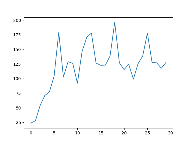
You can see that the reward is increasing, but it’s not quite stable yet. And this is one of the better runs too! There is a strange phenomenon that I’ve observed, which is that the rewards will go up and up and then suddenly drop to zero. This could be what people refer to as “catastrophic forgetting”, because the policy overfits to the environment. But strangely enough, my PyTorch implementation doesn’t suffer from this problem, even though the networks are almost identical.

But there you have it. Policy gradients! I hope you enjoyed this post and learned something new. Soon, we will explore many other algorithms, such as PPO, DQN, and many more. Stay tuned and I will see you in the next one.