Basics of Reinforcement Learning

2023-03-24

Reinforcement Learning is my favourite machine learning area and in this post, I will teach you about the basics of Reinforcement Learning (RL) and about the basic notation as well as other formulations in RL. Let’s get started!

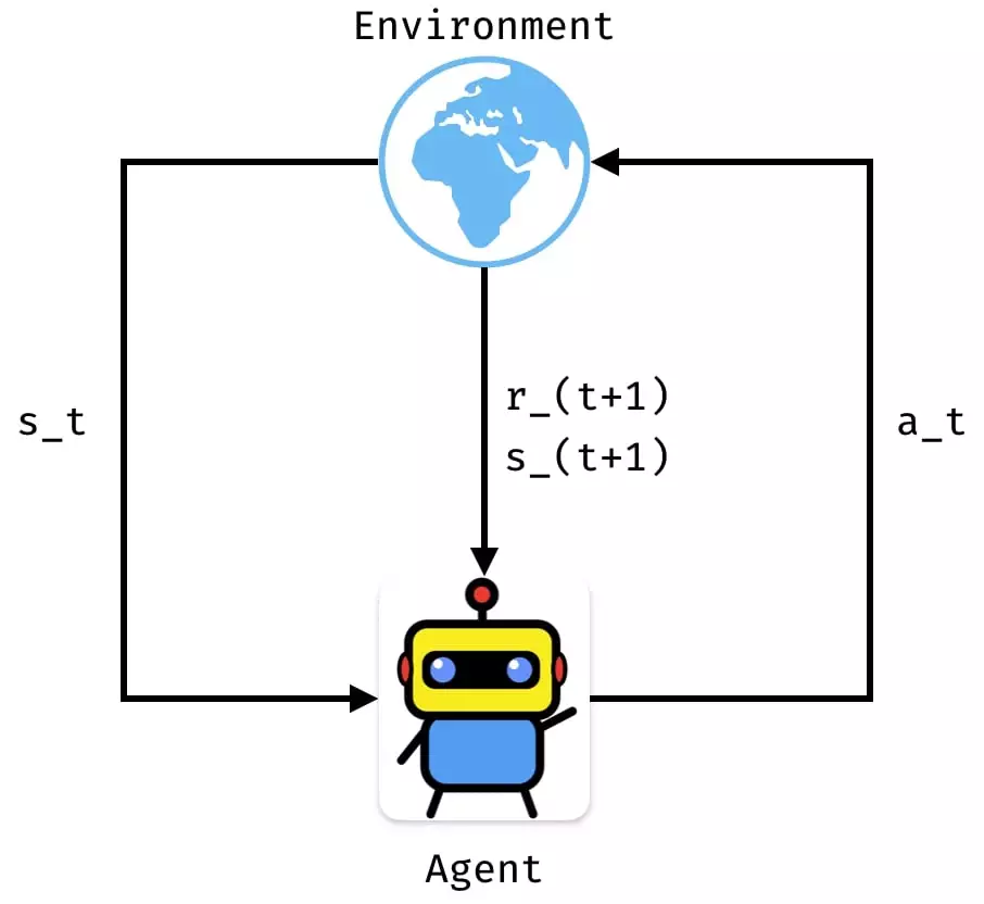
First, the general RL setting. In RL, we have an agent that interacts with an environment. The goal of the agent is to get as much reward as possible. At each time step, the agent can perform an action and receive a reward for that action. The figure below illustrates this.

RL Setting

When the agent interacts with the environment, it generates a so called trajectory. That trajectory is a list of state, action, reward tuples, i.e.:

\tau = ((s_0, a_0, r_0), \ldots, (s_i, a_i, r_i), \ldots (s_T, a_T, r_T))

A trajectory starts from timestep $t=0$ until $T$ which is the terminal timestep (i.e. the last timestep of the episode).

Given a trajectory, you can compute the return of the trajectory. How much return did you get from that trajectory? There are two types of returns you can compute: either the absolute return or the discounted return. The former is simply a sum of the rewards for every timestep:

R(\tau) = \sum_{t=0}^T = r_t

This is also called a finite horizon undiscounted reward. For the other case, you discount the return by some factor $\gamma \in [0, 1]$ and it’s referred to as infinite horizon discounted return. It’s defined as

R(\tau) = \sum_{t=0}^\infty = \gamma^t r_t

At each timestep, the agent sees the current state and decides what action to take. The action can either be deterministic or stochastic. If it’s deterministic, its written as

a_t = \mu_\theta(s_t)

and if it’s stochastic, then the action is sampled from a distribution, i.e.

a_t \sim \pi_\theta(s_t)

The $\theta$ is there to emphasise that those policies, whether deterministic or stochastic, usually are parameterised functions, such as neural networks and $\theta$ represents their parameters.

The action itself can either be discrete (e.g. press button A) or continious (e.g. actuate motor by 4.2). If it’s discrete, the logits given from the policy can be softmaxed to become probabilities and then simply sampled from. If the actions are continious, then the policy usually returns a Gaussian distribution (i.e. the mean and deviation). Then you simply use those to sample your action.

Let’s go back to our trajectory. What are the odds of getting a particular trajectory? It depends on the current policy of the agent of course, so let’s write that down:

P(\tau|\pi_\theta) = p_0(s_0)\prod_{t=0}^{T-1}P(s_{t+1}|a_t, s_t)\pi_\theta(a_t|s_t)

The equation above can be read as “the probability of getting trajectory $\tau$ given $\pi_\theta$ equals the probability of the initial state $s_0$ times the products of the probability to reach state $s_{t+1}$ given action $a_t$ and state $s_t$ times the probability to pick action $a_t$ given the current state $s_t$ .” As a useful shorthand, we can write $s' P(\cdot|s, a)$ , which reads as sampling the next state from the environment, given the current state and action.

With this, we can now define our objective function

J(\pi_\theta) = \int_{\mathcal{T}}P(\tau|\pi_\theta)R(\tau)

The objective function is also called the expected return:

J(\pi\theta) = \int_T P(\tau|\pi\theta)R(\tau) = \mathbb{E}_{\tau \sim \pi\theta} [R(\tau)]

And we’re trying to maximise the expected return! By the way, the best possible policy (and also the value functions - we’ll get to those) is written with a star, i.e. $\pi^*$

There are 2 more questions to answer:

How good is it to be in state $s_t$ and then follow my current policy?
How good is it to be in state $s_t$ , perform some arbitrary action $a_t$ and then follow my current policy?

The former is defined as the on-policy value function $V^\pi(s)$ :

V^\pi(s) = \mathbb{E}_{\tau \sim \pi}[R(\tau)|s_0 = s]

It’s called on-policy because the agent stays on the policy, i.e. it doesn’t “leave” the policy; it stays there. The latter is called the on-policy action-value function $Q^\pi(s, a)$ :

Q^\pi(s, a) = \mathbb{E}_{\tau \sim \pi}[R(\tau)|s_0 = s, a_0 = a]

Like with the optimal policy, both of the value functions have an optimal function, i.e.

V^*(s) = \max_\pi \mathbb{E}_{\tau \sim \pi}[R(\tau)|s_0 = s]

(which is the maximum expected return over all policies $\pi$ , given the initial state $s$ )

and

Q^*(s, a) = \max_\pi \mathbb{E}_{\tau \sim \pi}[R(\tau)|s_0 = s, a_0 = a]

(which is the maximum expected return for taking action $a$ in state $s$ and thereafter following the best policy $\pi$ )

The optimal action-value function is a bit more useful, because we can simply do this to get the optimal action:

a^*(s) = \arg \max_a Q^*(s, a)

The last bit of RL basics are the Bellman equations. These show a kind-of recursive property of the value functions, where the value of a state is the immediate return plus the discounted value of the next state. In other words:

V^\pi(s) = \mathbb{E}_{a \sim \pi, s' \sim P} [r(s, a) + \gamma V^\pi(s')]

V^*(s) = \mathbb{E}_{a \sim \pi, s' \sim P} [r(s, a) + \gamma V^*(s')]

And the same goes for the action-value function:

Q^\pi(s, a) = \mathbb{E}_{s' \sim P} [r(s, a) + \gamma \mathbb{E}_{a' \sim \pi} [Q^\pi(s', a')]] ,

Q^*(s, a) = \mathbb{E}_{s' \sim P} [r(s, a) + \gamma \max_{a'} Q^*(s', a')] ,

The last important part is the advantage function. It basically describes how good it is to pick action $a$ in state $s$ compared to the average action-value function (i.e. sampling actions from the policy). It’s defined as

A_\pi(s, a) = Q_\pi(s, a) - V_\pi(s)

And those are the basics of RL. In the next blog post, we will go one step further and implement REINFORCE (a policy gradient algorithm) and actually watch some agents in action! Stay tuned!